Association of vehicle emission charging zones with adult emergency hospital admissions: an interrupted time series analysis of the toxicity charge and Ultra Low Emission Zone in London, UK

Interesting comparative interrupted time series doing the rounds in the press at the moment.

Chamberlain, R. C., Hodsoll, J., Cai, C., Griffiths, C., Kelly, F., Beevers, S., Stewart, G., Blangiardo, M., Elliott, P., Davies, B., & Fecht, D. (2026). Association of vehicle emission charging zones with adult emergency hospital admissions: An interrupted time series analysis of the toxicity charge and Ultra Low Emission Zone in London, UK. Environment International, 213, 110324. https://doi.org/10.1016/j.envint.2026.110324

Whom and context again

I reread Mayne’s (2019) on contribution analysis today and see he also allows a “what works for whom”:

“… a more interesting and important contribution claim is around this evaluation question: How and why has the intervention (or component) made a difference, or not, and for whom?” (p. 174-5).

He also allows ToCs to describe contexts: “Using nested ToCs to unpack a complex intervention and its context has worked well in numerous situations…” (p. 178).

Mayne (2012) put context in the ToCs too: “External factors – context and rival explanations – influencing the intervention are assessed and are either shown not to have made a significant contribution or, if they did, their relative contribution is recognized.” (p. 273)

So there’s another theory-based brand with a “what works for whom in what context”, plus it uses generative causation 🙃

Of course I jest. Any approach can use generative causation, whether RCT or qualitative impact evaluation. Any approach can explore moderators of impact.

References

Mayne, J. (2012). Contribution analysis: Coming of age? Evaluation, 18(3), 270–280.

Mayne, J. (2019). Revisiting contribution analysis. Canadian Journal of Program Evaluation, 34(2), 171–191.

Extended two-way fixed effects

selectTWFE looks interesting: “Estimates both a vanilla two-way fixed effects (TWFE) model and an extended TWFE (ETWFE) model, then selects between them using Cochran’s Q test for heterogeneity. When ETWFE wins, reports the heterogeneity fraction (I-squared) and cohort-time estimates with empirical Bayes shrinkage and Bonferroni multiplicity correction.”

Dismantling evaluation brands

Thomas Aston (2026) has written a really interesting discussion of debates about what counts as realist evaluation and whether it is a unique kind of evaluation.

As I’ve written before (and Aston cites), I think theorising contexts, mechanisms, and outcomes (CMOs) is important, as is recognising a gap between theory, phenomena, and evidence. However, as Pawson (2024, p. 42) notes: “All [!] scientific investigation utilises explanations relating mechanisms and contexts to empirical patterns.” It’s science-as-usual. Pawson and Tilley know this – they acknowledge and cite earlier work. For example Pawson and Tilley (1997, p. 10) cite Palmer (1975, p. 150):

“Rather than ask, ‘What works for offenders as a whole?’ we must increasingly ask ‘Which methods work best for which types of offenders, and under what conditions or in what types of setting?'”

The link with science-as-usual is clear in Pawson and Tilley (2001, p. 324):

“We have argued that good evaluation is good social science. For us, this embraces the gallant aims of precision in articulation of theory, rigor in empirical testing, confederation in lines of inquiry, and cumulation in the body of findings. The ‘realist movement,’ of which we are a part, is often considered the brash upstart of the evaluation schools. In fact, it depends on these rather venerable ideas. The future, for us, thus lies in keeping faith with some of the grand old principles of social science and in not forgetting the hard-won lessons of the old studies.”

Evaluation method(ology) debates remind me of debates about psychological therapy brands, like CBT, psychodynamic, or humanistic approaches. Mick Power (2010) is an example therapist-academic who had a go at dismantling the brands, and pulled out graded exposure, transference, and challenging dysfunctional assumptions as example techniques that are used across a range of approaches. Others have done similar, e.g., the behavioural change technique taxonomy (Michie et al., 2013) extracts a long menu of approaches that can be combined to develop a programme.

I think evaluation would make faster progress if we routinely dismantled the big evaluation brands and asked of an apparently new and unique approach:

  1. Is it really unique?
  2. Who else has done similar?
  3. What is the approach an instance of?
  4. How could the approach be used in another type of evaluation?
  5. How could a technique be combined with another?

Westhorp and Feeny (2024) used this style of reasoning for realist evaluation, and showed how regression models with interaction terms can be used to test CMOs. Baumgartner and Falk (2023) explore regression-based alternatives to the Quine-McCluskey logical minimisation algorithm used in qualitative comparative analysis (QCA), closing the gap between QCA and statistics.

When it comes to questions of metaphysics, ask: what other approaches make the same or similar assumptions, e.g., concerning ontology and epistemology? For example, there’s a trace of the gap between mechanism and measure in questionnaire design: “operationalisation”, the process of developing a measure of, e.g., a psychological construct. This process begins with the premise that the phenomena are not directly observable. It’s psychometrics 101.

And this critical dismantling strategy applies to quantitative impact evaluation approaches too. Consider “synthetic controls” developed using the synthetic control method. They sounds unique and special; however, peek behind the curtain and they’re weighted averages, with weights estimated by balancing pre-intervention measurements of the outcome and covariates. So perhaps a comparison group developed using inverse probability of treatment weighting is also a “synthetic control”…? Maybe a t-test uses synthetic treatment and control groups, with unit weights…? Or consider entropy balancing, which, when targeting the ATT, is equivalent to inverse probability tilting (IPT; Słoczyński et al., 2025). The only difference is that entropy‑balancing weights sum to the comparison‑group sample size, whereas IPT weights sum to the intervention‑group sample size.

Build bridges between the methods and methodologies and they take up less space in your brain, making it easier to design robust evaluations and communicate clearly what you’re really setting out to do.

References

Aston, T. (2026). Evaluation blogs, podcasts, and webinars in the second half of 2025: Roundup review V. Evaluation.

Baumgartner, M., & Falk, C. (2023). Configurational Causal Modeling and Logic Regression. Multivariate Behavioral Research, 58(2), 292–310.

Michie, S., Richardson, M., Johnston, M., Abraham, C., Francis, J., Hardeman, W., Eccles, M. P., Cane, J., & Wood, C. E. (2013). The Behavior Change Technique Taxonomy (v1) of 93 Hierarchically Clustered Techniques: Building an International Consensus for the Reporting of Behavior Change Interventions. Annals of Behavioral Medicine, 46, 81–95.

Palmer, T. (1975). Martinson Revisited. Journal of Research in Crime and Delinquency, 12(2), 133–152.

Power, M. J. (2010). Emotion focussed cognitive therapy. John Wiley & Sons.

Słoczyński, T., Uysal, S. D., & Wooldridge, J. M. (2025). Covariate Balancing and the Equivalence of Weighting and Doubly Robust Estimators of Average Treatment Effects. IZA Institute of Labour Economics Discussion Paper, 18147.

Westhorp, G., & Feeny, S. (2025). Using surveys in realist evaluation. Evaluation Journal of Australasia, 25(1), 45–64.

Quasi-experiment sample size

Two papers caught my attention on sample‑size calculation: one for difference‑in‑differences designs (Hedberg & Hedges, 2026) and another for propensity score weighted designs (Liu et al., 2026).

Difference-in-differences (DiD)

Hedberg and Hedges (2026) have developed a method for estimating minimum detectable effect size (MDES) for DiD, including R code in an appendix. The approach takes account of variance explained by covariates (which could include fixed effects for units) and covariate imbalance. It also allows for unequal sample sizes. To run in reverse and estimate sample sizes, there’s a multitude of ways to get R to search across a range of sample sizes and minimise the difference between the achieved and target MDES.

Some things to bear in mind:

It handles both repeated cross-sectional and mixed between-within designs; for the latter, use fixed effects (so \(n-1\) covariates for \(n\) units) alongside an estimate of the variance explained. The parameters include the number of observations, not participants. So for a 2×2 design with pre and post measures from each participant, you will need to multiply the number of participants by 2.

There’s an error in the published code:

if (rho1 > 1) {
  V <- V*(1/(1-rho1^2))
}
if (rho2 > 1) {
  V <- V*(1-rho2^2)
}

Those rhos should never be over 1, and earlier checks won’t allow them to be. The code should check if they are over zero:

if (rho1 > 0) {
  V <- V*(1/(1-rho1^2))
}
if (rho2 > 0) {
  V <- V*(1-rho2^2)
}

I spotted this during testing: increasing the variance explained by covariates did not affect the MDES, and the results differed from the simulation checks. The corrected version resolves this, and the authors very kindly and promptly confirmed the fix. I understand that updated code will be available on the journal’s website soon. In the meantime, the edits noted above should address the issue.

Propensity score weighting

I had been using Austin’s (2021) work to approximate VIFs from c-statistics of propensity score models, which represent lack of overlap in propensity score distributions between groups. The resulting VIFs can then be used to inflate sample sizes estimated from standard power calculators.

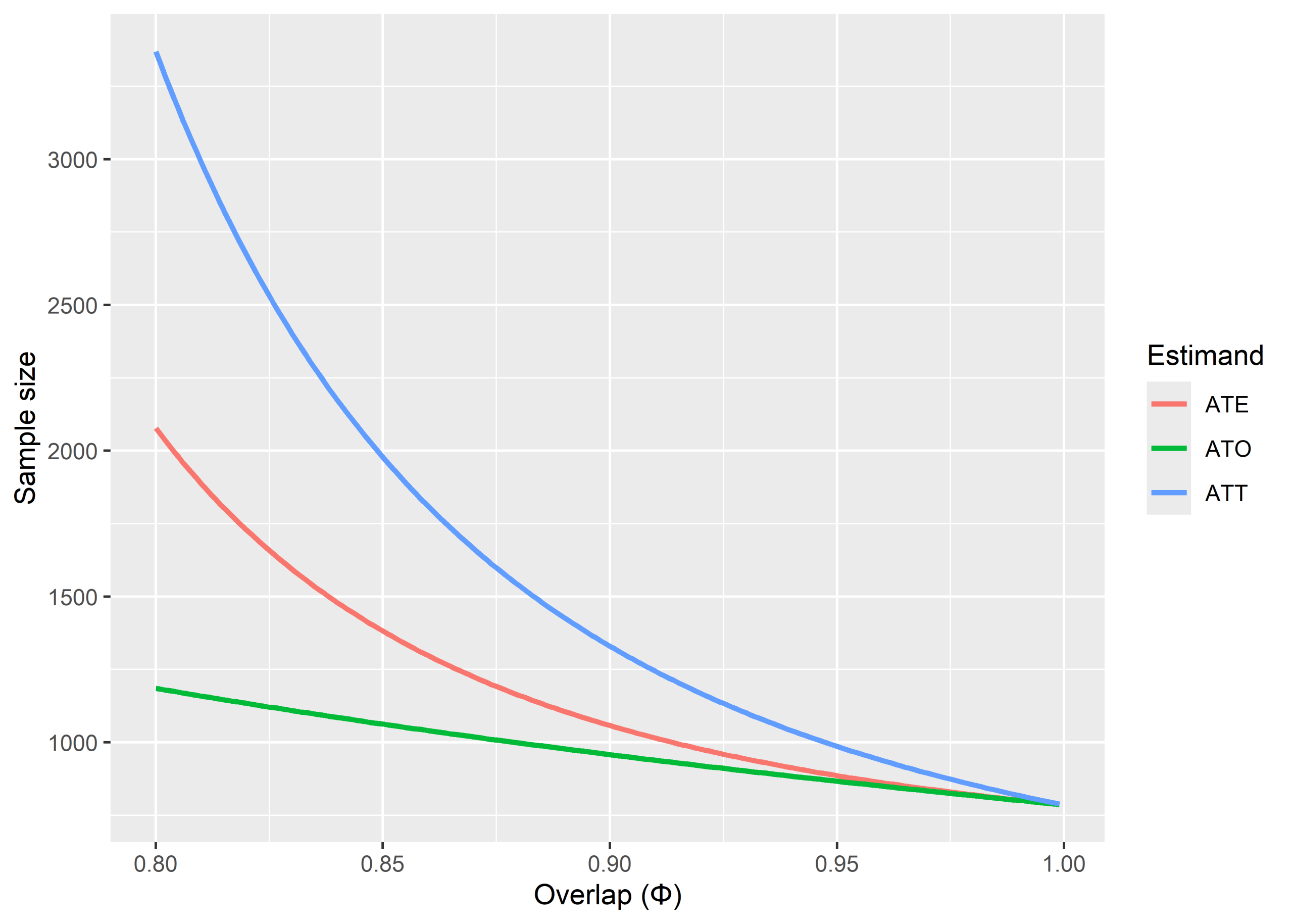
Liu, Yang, and Li (2026) have developed an alternative approach that does the sample size estimation in one go, depending on prevalence of the intervention, and an overlap parameter, \(\phi\), which is 1 with perfect overlap and decreases as the propensity score distributions separate. The approach has been implemented in the R package PSpower, which is on CRAN.

It’s speedy. Here’s an example with intervention prevalence at 50%, MDES 0.2, and varying the overlap from 80% to 99%, for the ATE, ATT, and ATO estimands. ATO is least affected by lack of overlap because it deliberately defines the estimand on the region where there is most overlap and down-weights observations that are far from there. ATO has a policy interpretation too: impact for people in the region of decisional equipoise.

References

Austin, P. C. (2021). Informing power and sample size calculations when using inverse probability of treatment weighting using the propensity score. Statistics in Medicine, 2, 1–14.

Liu, B., Yang, C., & Li, F. (2026). Sample size and power calculations for causal inference of observational studies (Version 5). arXiv, to appear in Annals of Statistics.

Hedberg, E. C., & Hedges, L. V. (2026). Computing Statistical Power for the Difference in Differences Design. Evaluation Review, 50(1), 149–180.

Bending evaluation timelines to meet policy deadlines

There is a simple formula for delivering evaluation findings in time to inform policymaking: \(T = S + R + D + I + A\).

Suppose that, for a programme to be considered effective, it must demonstrate a practically significant causal impact at least \(I\) months after the end of programme activities.

The programme duration is \(D\) months from the point at which a participant is enrolled in the evaluation.

Given recruitment rates, participants are enrolled over a period of \(R\) months to ensure sufficient numbers to achieve the required statistical power. The final participant therefore completes all programme activities \(R + D\) months after recruitment begins.

Study setup takes \(S\) months. This includes developing a theory of change, study design, developing surveys and topic guides, finalising the evaluation protocol, ethical approval, and recruiting study sites.

Analysis and reporting takes \(A\) months. This includes time waiting for administrative data requests to be fulfilled or for fieldwork to conclude, data management, statistical disclosure control and output clearance, peer review, and revisions.

The total study time is therefore \(T = S + R + D + I + A\) months. (You could add more steps, but it wrecks the anagram.)

For example, suppose the timeline is:

Setup3 months
Recruitment period6 months
Duration of the programme3 months
Impact time point6 months
Analysis and reporting3 months

The total duration \(T = 21\) months. So start the study 1 June 2026, it will report by 1 March 2028. And this evaluation only estimates impact at 6 months.

Suppose you want findings earlier than this as you need to inform an urgent policy decision. What could you do? Some options:

1. Analyse existing data for a similar programme, e.g., using meta-analysis of studies in a systematic review or quasi-experimental analysis of admin data. You can also gather implementation and process evidence to evaluate whether the current programme is being implemented correctly, even if you don’t have time to estimate impacts (use the review or secondary analysis of earlier similar programmes for that).

2. Investigate shorter-term outcomes, relying on existing evidence from similar programmes to argue that effects will endure. For example, it could be that you are really interested in impact at 10 years; however, the literature suggests that an outcome you can measure at 1 year is strongly correlated with the longer-term impact and the theory of change suggests it is an important link in the causal chain.

3. Shorten the programme duration, risking smaller impact and an underpowered study, so you may also need to boost the sample size, e.g., by lengthening the recruitment period.

4. Increase recruitment rates, e.g., by including more study sites or contacting more potential participants (depending on the nature of the programme).

5. Shorten the recruitment period, risking an underpowered study so you will likely have a wide confidence interval that straddles zero. Light a candle to guide interpretation.

6. Combine 4 and 5 to achieve the required sample size faster.

7. Run a simpler study, reducing setup, analysis, and reporting time. For example, you might measure only one or two key outcomes and conduct highly focused implementation and process evaluation.

8. Combine analysis of existing data with running a new evaluation: use option 1 (analyse existing data) to inform your policy design now, and also run the \(T\)-month evaluation to help out your future policy colleagues when they review the literature in a few years’ time.

9. Use time and relative dimensions in space-adjusted analysis to deliver the originally planned evaluation in time to feed into the policy decisions.

A policy evaluator about to embark on a three year evaluation that needs to report its findings in a few weeks’ time

Option 9 seems to be what policymakers expect. My preference would be to accept our spacetime structure and go for option 8 where possible (with the help of 2) or 1 if not. In any case, ensuring that evaluations can complete in time to inform policy requires long-term planning that is resilient to changes of PM, Ministers, and governments.

Thanks Edisa for inspiring a mild but crucial tweak to the variable names!

Applying a deontic logic to policy evaluation

One of the aims of policy evaluation is to support policymakers in making decisions. In practice, policymaking is shaped by coalitions of actors (Sabatier, 1988), including ministers and civil servants, opposition parties, professional bodies, charities, think tanks, campaigners, academics and journalists. Evaluation should aim to inform the deliberations of all these actors, not only those of whoever commissioned the work – regardless of whether it is remotely feasible to include them in a participatory process as part of the evaluation. Since each actor may hold normative values that clash with others’ values (understatement of the century), they may draw different conclusions about what should be done even when presented with the same evidence.

If the evidence produced by evaluators is to be relevant to a range of actors, we potentially need to reason about conflicting values. Deontic logics, which make it possible to reason about oughts, provide one way of structuring this reasoning. Given the complexities of applying deontic logics formally, as we will see shortly, and the large number of normative values involved, it is unlikely that evaluators will use them in a fully formal way. However, just as process tracing is informed by Bayesian logic (Bennett, 2009), I am curious whether informal reasoning about values can be informed by deontic logics. This post is a first go to find out.

There are many systems of deontic logic. A previous post ruled out standard deontic logic (SDL), which, confusingly, ceased to be standard in the late 1960s (Parent & Torre, 2018, p. 20). An alternative I’d like to explore is Horty’s (2012) approach, a prioritised default logic, which has the following key characteristics:

  1. Classical logic is monotonic, in the sense that adding more premises to an argument can never lead to the retraction of a conclusion: either the set of conclusions stays the same or grows (note the parallel with monotonic functions). Horty’s logic is nonmonotonic, meaning that it does allow conclusions to be withdrawn. The classic example concerns a bird named Tweety. All birds fly, so we conclude that Tweety flies. However, if we subsequently learn that Tweety is a penguin, we revise that conclusion and conclude that Tweety doesn’t fly.
  2. Horty’s nonmonotonic logic is implemented using default rules (defaults for short), written as \(\phi \rightarrow \psi\), which are read as: if we have established \(\phi\), then we should conclude \(\psi\) by default (for example, that birds fly). This inference can be overruled if another default supports a contradictory conclusion (for example, that penguins do not fly).
  3. Defaults represent reasons for believing things (e.g., Tweety can’t fly because Tweety is a Penguin) or reasons for doing things (e.g., meeting a friend for lunch because we promised to).
  4. Some default rules have higher priority than others, e.g., if \(\delta_1\) and \(\delta_2\) are two defaults, then \(\delta_1 > \delta_2\) means that \(\delta_1\) has higher priority than \(\delta_2\), so can overrule it. This might be due to the rule being more specific, e.g., if we’re reasoning about penguins we should prioritise defaults about penguins rather than about birds more generally. When defaults refer to normative values, the priorities determine which values are more important than others.
  5. The system therefore makes it possible to reason about moral conflicts. One of Horty’s examples involves a promise to meet a friend for lunch and a moral obligation to save a drowning child encountered en route to lunch. A reasonable ordering on defaults representing these norms is that saving a drowning child takes priority over fulfilling a lunch promise, so the logic concludes that the child should be rescued.

To illustrate how this works, let’s explore the following simplified example:

  • An evaluation has shown that a programme leads to an outcome valued by a policymaker: \(P\).
  • The same evaluation has shown an unanticipated harmful consequence of the programme that was not considered by policymakers or evaluators at the outset, but was highlighted by service users: \(H\).
  • If the valued outcome is found, then we should roll out the programme nationally: \(d_1 = P \rightarrow R\).
  • If harmful outcomes are found, then it should not be rolled out nationally: \(d_2 = H \rightarrow \neg R\).

We could complicate this further by introducing differences in the quality of evidence. For example, \(P\) might have been established through a rigorous impact evaluation, whereas \(H\) might have been identified through qualitative interviews with a small sample – a common way in which unintended consequences are discovered. However, to keep the discussion simple, let’s assume that there is no difference in the quality of evidence.

How do we evaluate evidence using Horty’s prioritised default logic? Since it is a logic, the rules are all formally defined, and applying them in practice can be challenging. Horty’s (2012) explanation spans several chapters. Here follows a concise summary; refer to the original text for fuller explanation and worked examples.

A default theory consists of three elements, which for the example above would be:

  1. \(\mathcal{W} = \{ P, H \}\) is the starting point for our inferences, representing the evidence found by the evaluation and any background assumptions. This would include relationships between the variables, which we don’t have in our simplified policy example. For the Tweety example, it would include that penguins are birds.
  2. \(\mathcal{D} = \{ d_1, d_2 \}\) is the set of defaults described above. For a default \(\phi \rightarrow \psi\), \(\phi\) is the premise and \(\psi\) the conclusion. We can refer to the premises and conclusions of a default or set of defaults, \(\Delta\), using \(\text{premise}(\Delta)\) and \(\text{conclusion}(\Delta)\).
  3. \(<\) is the ordering on the defaults, which specifies which take precedence over others. This is a partial ordering, in the sense that some or all defaults may have the same precedence. Let’s begin with no ordering, so the defaults concerning desired (\(d_1\)) and harmful (\(d_2\)) outcomes have equal importance.

To draw inferences, we need to consider one or more scenarios: these are a subset of the defaults, \(S \subseteq \mathcal{D}\). A scenario could include some, all, or none of the defaults. Binding defaults are defaults in the full theory such that the following conditions hold for a scenario:

  1. The default \(\delta \in \mathcal{D}\) is triggered, in the sense that its premise logically follows from the background theory and conclusions of the defaults in the scenario: \(\mathcal{W} \cup \text{conclusion}(S) \vdash \text{premise}(\delta)\).
  2. The default \(\delta \in \mathcal{D}\) is not conflicted, i.e., its conclusion does not contradict the background theory and scenario: it is not the case that \(\mathcal{W} \cup \text{conclusion}(S) \vdash \neg \text{conclusion}(\delta)\).
  3. The default \(\delta \in \mathcal{D}\) is not defeated by another default in the theory, i.e., there is no triggered default \(\delta^\prime > \delta\) such that \(\delta^\prime\) and \(\delta\) arrive at contradictory conclusions: it is not the case that \(\mathcal{W} \cup \text{conclusion}(\delta^\prime) \vdash \neg \text{conclusion}(\delta)\).

A scenario, \(S \subseteq \mathcal{D}\), is a proper scenario if it doesn’t include any extra defaults in \(\mathcal{D}\) that aren’t binding and doesn’t miss out any defaults that are binding. A proper scenario includes the good reasons for drawing an inference, and is what we (or an algorithm) are trying to find. More than one scenario may be proper.

We want to know what logically follows from each proper scenario, known as the extension, \(\mathcal{E}\), since it extends beyond the background theory and default rules to what they logically imply. This is a set of conclusions, defined

\(\mathcal{E} = \text{Th}\bigl(\mathcal{W} \cup \text{conclusion(S)}\bigr)\),

where \(\text{Th}(\Gamma)\) is the set of propositions, \(\phi\), such that \(\Gamma \vdash \phi\), i.e., every proposition that logically follows from \(\Gamma\).

Finally, how do we conclude that some proposition \(\phi\) ought to be the case, \(\mathsf{O} \phi\)? There are two ways to do this, depending on how we deal with conflicts:

  1. Conflict account: \(\mathsf{O} \phi\) follows if and only if \(\phi\) is included in the extension of at least one proper scenario.
  2. Disjunctive account: \(\mathsf{O} \phi\) follows if and only if \(\phi\) is included in extensions of all proper scenarios.

It is straightforward to find the proper scenarios for our example. We know both defaults are triggered, since the evidence \(\mathcal{W} = \{ P, H \}\), and the defaults are:

\(\displaystyle \begin{aligned}
d_1 &= P \rightarrow R \\
d_2 &= H \rightarrow \neg R
\end{aligned}\)

The conclusions of the two defaults contradict each other (\(R\) and \(\neg R\)), so if we included them both in a scenario they would be conflicted. Neither of the defaults could be defeated by the other since we have not put an ordering on them, and defeat requires an ordering. So there are two proper scenarios: \(\{ d_1 \}\) and \(\{ d_2 \}\), and two sets of extensions, call them \(\mathcal{E}_1\) and \(\mathcal{E}_2\).

  • \(\mathcal{E}_1\) includes \(\{ P, H, R \}\), so we can conclude \(\mathsf{O} R\).
  • \(\mathcal{E}_2\) includes \(\{ P, H, \neg R \}\), so we can conclude \(\mathsf{O} \neg R\).

Under the conflict account, this means we have two oughts: \(\mathsf{O} R\) and \(\mathsf{O} \neg R\). Note the extensions \(\mathcal{E}_1\) and \(\mathcal{E}_2\) both also include \(R \lor \neg R\) (using disjunction introduction), so by the disjunctive account we can conclude \(\mathsf{O}(R \lor \neg R)\). Therefore, with no ordering on the defaults, we can only say that we either ought to roll out the programme or not roll it out. Not particularly helpful!

To arrive at a decision, we need to put an ordering on the defaults. We could reason that an important normative value is first do no harm, which could be formalised as \(d_2 > d_1\). In this case, the only proper scenario is \(\{ d_2 \}\). This is because a proper scenario cannot have any defeated defaults, and in scenarios \(\{ d_1 \}\) and \(\{ d_1, d_2 \}\), \(d_1\) would be defeated by \(d_2\). We can’t use the empty scenario since it excludes binding defaults, so it is not a proper scenario. The extension of the proper scenario leads to the conclusion \(\mathsf{O} \neg R\): we ought not roll out the programme.

I noted earlier that SDL is ruled out as an appropriate logic for deontic reasoning. It does not, for example, handle conflicts in obligations. However, there’s something slightly puzzling about how Horty (2012) derives oughts: if \(\phi\) is in the extension of a scenario, we can conclude \(\mathsf{O} \phi\) for that scenario. But defaults can include non-deontic conclusions, such as the inference that penguins do not fly. It seems odd to move from this belief to the conclusion that penguins ought not fly. Fuhrmann (2017) suggests instead ditching Horty’s move from extensions to oughts and supplementing the system with SDL. Our original set of defaults would then be:

\(\displaystyle \begin{aligned}
d_1 &= P \rightarrow \mathsf{O} R \\
d_2 &= H \rightarrow \mathsf{O} \neg R
\end{aligned}\)

The idea is that instead of using classical logical consequence for building extensions, we use SDL. An extension of a scenario can then include an ought “for free”, since default conclusions can include oughts. The conflict and disjunctive accounts still work for examples Fuhrmann tries, yielding reasonable inferences, and we also still have the very helpful machinery of default logic. I don’t know whether adding SDL introduces other problems, though.

Does Horty’s prioritised default logic, perhaps supplemented with SDL, help evaluation? Firstly, it offers a deontic logic that formalises some elements of evaluative thinking. Even if we do not use it in a fully formal way, it provides clues about what evaluative thinking needs to include and highlights some of the issues that may arise. For example, we need to anticipate what the potential findings might be and how different normative values may lead to different evaluative judgements.

Secondly, it suggests that one way to do this is through default rules – formally or informally specified – with orderings where possible to reduce the number of conflicting conclusions. This allows some defaults to take priority over others. The justifications for that ordering lie outside the logic itself and form part of what coalitions of actors will debate.

Finally, as alluded to above, we also need an ordering on the evidence, and we need to ensure evaluations are designed so that, for example, if harms are identified, evidence of those harms cannot simply be dismissed on the grounds that the evidence is of insufficient quality. For example, suppose we have evidence from an impact evaluation (e.g., a quasi-experiment) of no harms (\(\neg H_I\)) and evidence from a process evaluation (e.g., qualitative interviews) of harms (\(H_P\)). We could setup defaults to interpret this evidence as:

\(\displaystyle \begin{aligned}
i_1 &= H_I \rightarrow H \\
i_2 &= \neg H_I \rightarrow \neg H \\
p_1 &= H_P \rightarrow H \\
p_2 &= \neg H_P \rightarrow \neg H
\end{aligned}\)

where \(H\) means we have inferred the programme has caused harm. Order the defaults so that \(i_x > p_x\) for \(x = 1,2\). This would mean that with conflicting evidence of harms, the impact evaluation evidence would always trump the process evaluation evidence. So, given the evidence \(\{ \neg H_I, H_P \}\), the conclusion would be no harm, \(\neg H\). This mirrors how process evaluation evidence of perceived impact is often, in practice, defeated by impact evaluation evidence of no impact. These interpretations can be anticipated before any data is collected and feed into the design of an evaluation.

I think it is unrealistic to expect an evaluation to settle debates about normative values, for the reasons explored in a previous post. However, deontic logic could help us think through what evidence needs to be produced to support others when they have those debates, making explicit both the assumed priorities among different forms of evidence and the ways in which this evidence is taken to justify particular policy decisions.

References

Bennett, A. (2009). Process Tracing: A Bayesian Perspective. In J. M. Box-Steffensmeier, H. E. Brady, & D. Collier (Eds), The Oxford Handbook of Political Methodology (pp. 702–721). Oxford University Press.

Fuhrmann, A. (2017). Deontic Modals: Why Abandon the Default Approach. Erkenntnis, 82(6), 1351–1365.

Horty, J. F. (2012). Reasons as defaults. Oxford University Press. (Final version preprint available here.)

Parent, X., & Torre, L. van der. (2018). Introduction to Deontic Logic  and Normative Systems. College Publications.

Sabatier, P. A. (1988). An advocacy coalition framework of policy change and the role of policy-oriented learning therein. Policy Sciences, 21, 129–168.