Quasi-experiment sample size

Two papers caught my attention on sample‑size calculation: one for difference‑in‑differences designs (Hedberg & Hedges, 2026) and another for propensity score weighted designs (Liu et al., 2026).

Difference-in-differences (DiD)

Hedberg and Hedges (2026) have developed a method for estimating minimum detectable effect size (MDES) for DiD, including R code in an appendix. The approach takes account of variance explained by covariates (which could include fixed effects for units) and covariate imbalance. It also allows for unequal sample sizes. To run in reverse and estimate sample sizes, there’s a multitude of ways to get R to search across a range of sample sizes and minimise the difference between the achieved and target MDES.

Some things to bear in mind:

It handles both repeated cross-sectional and mixed between-within designs; for the latter, use fixed effects (so \(n-1\) covariates for \(n\) units) alongside an estimate of the variance explained. The parameters include the number of observations, not participants. So for a 2×2 design with pre and post measures from each participant, you will need to multiply the number of participants by 2.

There’s an error in the published code:

if (rho1 > 1) {
  V <- V*(1/(1-rho1^2))
}
if (rho2 > 1) {
  V <- V*(1-rho2^2)
}

Those rhos should never be over 1, and earlier checks won’t allow them to be. The code should check if they are over zero:

if (rho1 > 0) {
  V <- V*(1/(1-rho1^2))
}
if (rho2 > 0) {
  V <- V*(1-rho2^2)
}

I spotted this during testing: increasing the variance explained by covariates did not affect the MDES, and the results differed from the simulation checks. The corrected version resolves this, and the authors very kindly and promptly confirmed the fix. I understand that updated code will be available on the journal’s website soon. In the meantime, the edits noted above should address the issue.

Propensity score weighting

I had been using Austin’s (2021) work to approximate VIFs from c-statistics of propensity score models, which represent lack of overlap in propensity score distributions between groups. The resulting VIFs can then be used to inflate sample sizes estimated from standard power calculators.

Liu, Yang, and Li (2026) have developed an alternative approach that does the sample size estimation in one go, depending on prevalence of the intervention, and an overlap parameter, \(\phi\), which is 1 with perfect overlap and decreases as the propensity score distributions separate. The approach has been implemented in the R package PSpower, which is on CRAN.

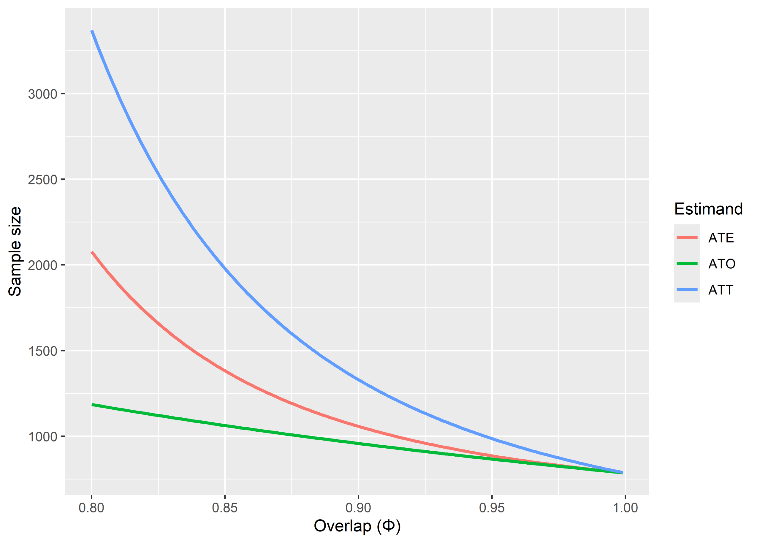
It’s speedy. Here’s an example with intervention prevalence at 50%, MDES 0.2, and varying the overlap from 80% to 99%, for the ATE, ATT, and ATO estimands. ATO is least affected by lack of overlap because it deliberately defines the estimand on the region where there is most overlap and down-weights observations that are far from there. ATO has a policy interpretation too: impact for people in the region of decisional equipoise.
References

Austin, P. C. (2021). Informing power and sample size calculations when using inverse probability of treatment weighting using the propensity score. Statistics in Medicine, 2, 1–14.

Liu, B., Yang, C., & Li, F. (2026). Sample size and power calculations for causal inference of observational studies (Version 5). arXiv, to appear in Annals of Statistics.

Hedberg, E. C., & Hedges, L. V. (2026). Computing Statistical Power for the Difference in Differences Design. Evaluation Review, 50(1), 149–180.

Entropy balancing and inverse probability tilting

Something fun (Słoczyński et al., 2025, p. 3, footnote 1):

“IPT [inverse probability tilting] coincides with Hainmueller’s (2012) entropy balancing estimator when the propensity score is estimated with the logit model”.

(It just holds for ATT.) The picture below illustrates the correspondence, using the Lalonde (1986) dataset (in the cobalt package in R). I computed (knitted R here) the weights using the WeightIt package (Greifer, 2025). Since we’re aiming for ATT, the intervention group weights are all equal to 1, so I’ve omitted them from the graph.

The weights are perfectly correlated and the effective sample sizes are the same. They are scaled differently, though (in the WeightIt implementation at least – need to wade into the original papers): entropy weights sum to the comparison group sample size and IPT weights sum to the intervention group sample size.

References

Greifer, N. (2025). WeightIt: Weighting for Covariate Balance in Observational Studies (version 1.5.0) [R Package].

Słoczyński, T., Uysal, S. D., & Wooldridge, J. M. (2025). Covariate Balancing and the Equivalence of Weighting and Doubly Robust Estimators of Average Treatment Effects. IZA Institute of Labour Economics Discussion Paper, 18147.

Fei Wan (2025) on propensity score matching

Quasi-experimentalists will be familiar with King and Nielsen’s (2019) landmark paper, Why Propensity Scores Should Not Be Used for Matching. This specifically critiqued the use of propensity scores for matching; other common uses of propensity scores, such as inverse probability weighting, were not affected. An interesting paper has appeared by Fei Wan (2025) critiquing King and Nielsen’s findings.

Fei Wan’s targets include:

  1. The inappropriateness of using an average pairwise covariate distance between treated and closest comparison match to evaluate PSM. Distances are always nonnegative so can’t take account of positive and negative differences averaging out. It’s already known that two observations with the same propensity score are likely to have different covariate values, but it’s ok if they are random.
  2. King and Nielsen used a cherry-picking approach for model selection, trying 512 different specifications and selecting the one that yields the largest average treatment estimate. This is just poor analysis practice.

Fei Wan recommends machine learning approaches to estimate propensity scores, rather than the common use of logistic regression.

Lots more to digest in this…

References

King, G., & Nielsen, R. (2019). Why Propensity Scores Should Not Be Used for Matching. Political Analysis, 27(4), 435–454.

Wan, F. (2025). Propensity Score Matching: Should we use it in designing observational studies? BMC Medical Research Methodology, 25(1), 25.

Propensity score analysis with baseline measure of outcome

Mild headache in this new simulation study by Peter Austin of propensity score matching/weighting studies where you have a baseline measurement of the outcome variable – a useful thing to balance as it’s often highly correlated with outcome.

For ATE, the recommendations make sense: include the baseline in the propensity model and then, for what are often called doubly robust approaches, include baseline again as a covariate in the outcome model.

For ATT, the findings are not what I would have expected. Austin’s recommendation for best standard errors is to exclude the baseline from the propensity model and analyse change from baseline in the outcome model 😱:

“… recommendations for the analysis of RCTs with baseline measurements of the follow-up variable do not reflect perfectly what we observed in the context of the analysis of observational studies using propensity score methods. We found that the analysis of change from baseline using a propensity score that excluded the baseline value of the follow-up variable tended to result in the most precise estimates of treatment effect. However, we did observe that, when using weighting, the use of ANCOVA in conjunction with a propensity score model that included the baseline value of the follow-up variable tended to perform well.”

One to read properly to see what’s going on. Would be interested in your thoughts.

References

Austin, P. (2024). Propensity Score Analysis With Baseline and Follow-Up Measurements of the Outcome Variable. Pharmaceutical Statistics. Early view.

Sample size determination for propensity score weighting

If you’re using propensity score weighting (e.g., inverse probability weighting), one question that will arise is how big a sample you need.

Solutions have been proposed that rely on a variance inflation factor (VIF). You calculate the sample size for a simple design and then multiply that by the VIF to take account of weighting.

But the problem is that it is difficult to choose a VIF in advance.

Austin (2021) has developed a simple method (R code in the paper) to estimate VIFs from c-statistics (area under the curve; AOC) of the propensity score models. These c-statistics are often published.

A larger c-statistic means a greater separation between treatment and control, which in turn leads to a larger VIF and requirement for a larger sample.

Picture illustrating different c-statistics.

The magnitude of the VIF also depends on the estimand of interest, e.g., whether average treatment effect (ATE), average treatment effect on the treated (ATET/ATT), or average treatment effect where treat and control overlap (ATO).

References

Austin, P. C. (2021). Informing power and sample size calculations when using inverse probability of treatment weighting using the propensity score. Statistics in Medicine.