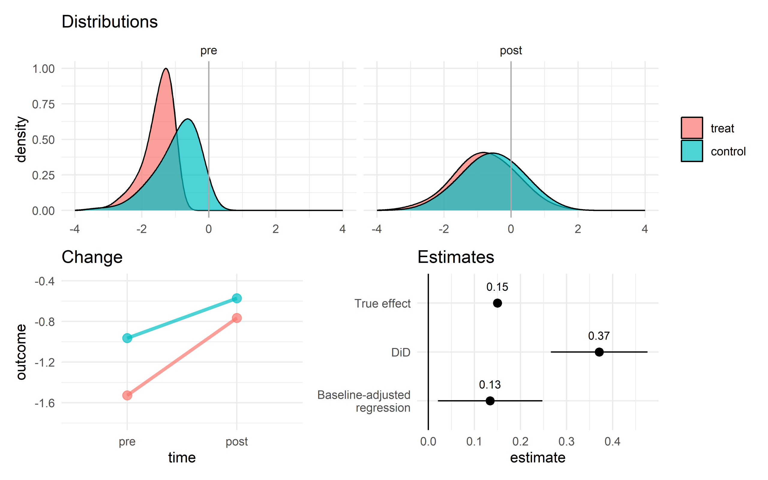
In another episode of, I wonder how well just regressing outcome on intervention group and baseline will do…? Here’s a scenario which breaks the diff-in-diffs parallel trends assumption using regression to the mean.
The treatment group observations were selected so they’re further below the mean at baseline than the control group observations, so by regression to the mean alone, the treat group will show more change. (Pre-post correlation 0.6 in the population, before selection.)
The DiD model was the usual 2×2 approach with participant fixed effects, which control for time-invariant effects that will not save us here.
The baseline-adjusted model regresses outcome on group and baseline.
The only confounder is baseline.
See Ryan (2018) for discussion of some of the muddles in the DiD lit on these kinds of effects.
References
Ryan, A. M. (2018). Well‐Balanced or too Matchy–Matchy? The Controversy over Matching in Difference‐in‐Differences. Health Services Research, 53(6), 4106–4110.
selectTWFE looks interesting: “Estimates both a vanilla two-way fixed effects (TWFE) model and an extended TWFE (ETWFE) model, then selects between them using Cochran’s Q test for heterogeneity. When ETWFE wins, reports the heterogeneity fraction (I-squared) and cohort-time estimates with empirical Bayes shrinkage and Bonferroni multiplicity correction.”
Two papers caught my attention on sample‑size calculation: one for difference‑in‑differences designs (Hedberg & Hedges, 2026) and another for propensity score weighted designs (Liu et al., 2026).
Difference-in-differences (DiD)
Hedberg and Hedges (2026) have developed a method for estimating minimum detectable effect size (MDES) for DiD, including R code in an appendix. The approach takes account of variance explained by covariates (which could include fixed effects for units) and covariate imbalance. It also allows for unequal sample sizes. To run in reverse and estimate sample sizes, there’s a multitude of ways to get R to search across a range of sample sizes and minimise the difference between the achieved and target MDES.
Some things to bear in mind:
It handles both repeated cross-sectional and mixed between-within designs; for the latter, use fixed effects (so \(n-1\) covariates for \(n\) units) alongside an estimate of the variance explained. The parameters include the number of observations, not participants. So for a 2×2 design with pre and post measures from each participant, you will need to multiply the number of participants by 2.
There’s an error in the published code:
if (rho1 > 1) {
  V <- V*(1/(1-rho1^2))
}
if (rho2 > 1) {
  V <- V*(1-rho2^2)
}
Those rhos should never be over 1, and earlier checks won’t allow them to be. The code should check if they are over zero:
if (rho1 > 0) {
  V <- V*(1/(1-rho1^2))
}
if (rho2 > 0) {
  V <- V*(1-rho2^2)
}
I spotted this during testing: increasing the variance explained by covariates did not affect the MDES, and the results differed from the simulation checks. The corrected version resolves this, and the authors very kindly and promptly confirmed the fix. I understand that updated code will be available on the journal’s website soon. In the meantime, the edits noted above should address the issue.
Propensity score weighting
I had been using Austin’s (2021) work to approximate VIFs from c-statistics of propensity score models, which represent lack of overlap in propensity score distributions between groups. The resulting VIFs can then be used to inflate sample sizes estimated from standard power calculators.
Liu, Yang, and Li (2026) have developed an alternative approach that does the sample size estimation in one go, depending on prevalence of the intervention, and an overlap parameter, \(\phi\), which is 1 with perfect overlap and decreases as the propensity score distributions separate. The approach has been implemented in the R package PSpower, which is on CRAN.
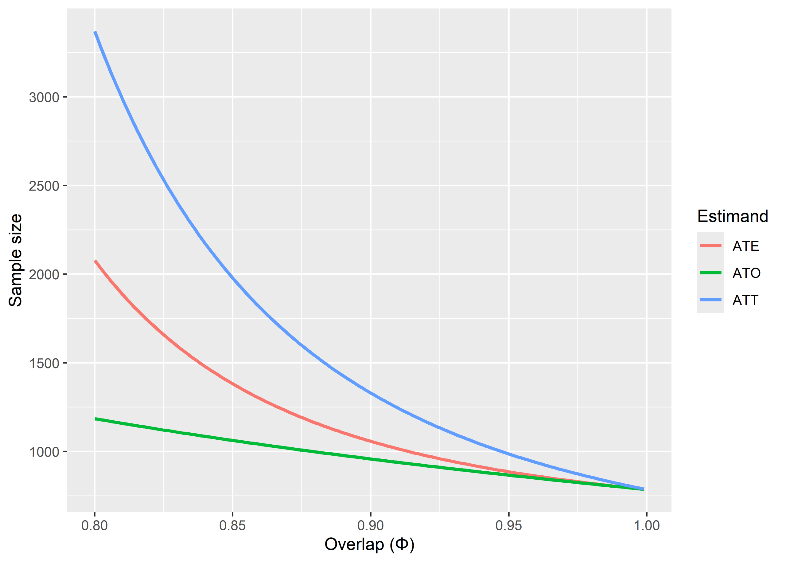
It’s speedy. Here’s an example with intervention prevalence at 50%, MDES 0.2, and varying the overlap from 80% to 99%, for the ATE, ATT, and ATO estimands. ATO is least affected by lack of overlap because it deliberately defines the estimand on the region where there is most overlap and down-weights observations that are far from there. ATO has a policy interpretation too: impact for people in the region of decisional equipoise.
Social policy evaluation inherits concepts from multiple disciplines, and somewhere along the way many of them have become muddled. The list below sketches what I think are seven of the most harmful myths.
1. “Counterfactual” is a synonym for control/comparison group
There is a long history of research on counterfactual reasoning in the absence of a control group. For example, analyses of how people should and can determine the truth of a counterfactual conditional such as “If Oswald had not killed Kennedy, no one else would have” or “If I’d left the house earlier, I’d have caught that bus” (e.g., Adams, 1970; Halpern, 2015). We ponder counterfactuals like these all the time without running RCTs.
The evaluation literature has also considered how counterfactuals can be used without a comparison group (e.g., White, 2010) – including with qualitative evidence (e.g., Reichardt, 2022). In evaluation, the counterfactuals are conditionals like, “If intervention group students hadn’t been offered the mentoring programme, x% fewer would have passed their GCSEs.”
Some evidence for counterfactual outcomes is more robust than others. One example analysed by Reichardt (2022) involves asking programme participants what they think would have happened if they had not taken part in the programme. Their ability to answer this depends on their capacity for counterfactual reasoning, which may be limited for some programmes. For instance, many people believe that homeopathy is effective, even though its remedies are so highly diluted that they contain no active ingredients and cannot have any biological effect (Ernst, 2005). Counterfactual reasoning based on such beliefs could therefore falsely conclude that a programme caused improvements that would have occurred anyway.
Quantitative designs can be used to estimate counterfactual outcomes without a comparison group. One example is interrupted time series, which uses trends in pre-intervention outcomes to estimate post-intervention counterfactual outcomes. This is illustrated below:
The standard analysis estimates whether introducing the intervention shifted the outcome and whether it changed the slope, both relative to the inferred counterfactual outcomes.
When a comparison group is used to estimate counterfactual outcomes, it is a factual group – it consists of real data from real people. If it were a counterfactual group, it couldn’t be used to estimate anything. This is why I avoid the term “counterfactual group”.
2. RCTs only estimate overall average effects
If you think causal effects may vary by, e.g., participant characteristics or the context they are in, then you can test this by using moderator analysis and obtain estimates for each group. For example, trials funded by the Education Endowment Foundation usually investigate whether the magnitude of a programme’s effects differ for students who are eligible for free school meals – a proxy for socioeconomic disadvantage (e.g., Takala, et al., 2025). Westhorp and Feeny (2024) suggest using moderator analysis to test the effect of context in realist evaluations (see also Myth 4 below).
One challenge is that when testing for moderator effects for variables with a large number of levels – for example, in intersectional analyses of gender and ethnicity – models can become unwieldy very quickly. The UK census, for example, includes 19 ethnicities and 6 genders (including cis and trans identities). That results in 114 possible combinations. A promising solution is multilevel analysis of individual heterogeneity and discriminatory accuracy – MAIHDA, for short (Merlo, 2018).
3. (Trialists believe that) RCTs don’t need a programme theory
Individual causal effects are defined as the difference between what a person’s outcome would be following intervention and what it would be following control. We can’t observe this within‑person difference because each participant only experiences one condition. With random assignment, however, the average outcome of those in the intervention group minus the average outcome of those in the control group (a between‑person difference) provides an unbiased estimate of the average of individual causal effects (averages of the unmeasureable within-person differences) – even without any covariates. That’s the great thing about RCTs.
RCTs still need theory. How do you choose a control group? Outcome variables? How do you interpret estimated causal effects, i.e., what the difference between intervention and control outcomes means? Chen and Rossi (1980) explain how theory-based (what they call theory-driven) RCTs that include theory-informed covariates yield more precise estimates of effects (reducing the probability of Type II error), even though those covariates are not needed to control Type I error. That’s why sample size calculators ask how much variance in outcomes is thought to be explained by covariates. RCTs can also test mechanisms of change, e.g., using mediation analysis or through factorial designs.
A related myth is that trialists believe reality consists of variables. Paley and Lilford (2011, pp. 956-7) dispute this:
The view attributed to positivism, that reality is fragmented into variables, is a straw man. No one believes it, and classification into types is something that all researchers, both quantitative and qualitative, do. Variables are a product of measurement procedures; they are not part of the structure of reality.
Good theories of change go beyond the variables to discuss people and other entities and what they do (see Myth 6). Variables operationalise aspects of these.
Incidentally, trialists don’t need to be positivists either. Bogen and Woodward (1988) provide an accessible discussion of how to think about the relationship between theory and observed phenomena without falling into positivism.
4. Realist evaluation is a distinct type of evaluation
What people do in practice when they say they are conducting a realist evaluation or “using realist principles” often makes sense, and Pawson and Tilley’s work has helped bring theory to the fore in evaluation (I put at least one reading of theirs on my social theorising course when I was an academic). But the idea that you need a realist evaluation to find out “what works best for whom in what context” or to describe change in terms of context, mechanisms, and outcomes, is just absurd. Many evaluation approaches do this.
Paul (1967, p. 111) offers an earlier example of the what works for whom logic:
[…] the question towards which all outcome research should ultimately be directed is the following: What treatment, by whom, is most effective for this individual with that specific problem, and under which set of circumstances?
Pawson and Tilley (1997, p. 10) cite Palmer (1975, p. 150), who uses similar logic:
Rather than ask, “What works for offenders as a whole?” we must increasingly ask “Which methods work best for which types of offenders, and under what conditions or in what types of setting ?”
School climate research offers one example of contextual factors: the physical characteristics of schools; the formal and informal rules that operate within them; and the norms, beliefs, and values at play (Anderson, 1982). RCTs have examined the extent to which school climate moderates programme effects – i.e., how outcomes depend on the settings in which programmes are delivered (e.g., Low & Van Ryzin, 2014) – as well as the mediating role of climate, where a programme changes aspects of school climate and these changes help to explain its effects (e.g., Singla et al., 2021).
My reading of Pawson and Tilley (1997) and Pawson (2024) is that they’re introducing the scientific method and philosophy of science to evaluators who don’t have a formal training in a science. The ideas apply to any form of evaluation. For example, Pawson (2024, p. 42) argues that
All scientific investigation utilises explanations relating mechanisms and contexts to empirical patterns.
Science is not simply about observing regularities or estimating average causal effects. It is about explaining why observed patterns occur, how they are produced, and under what conditions they hold. This logic applies whether you are running an RCT, conducting a qualitative impact evaluation, or analysing administrative data using a quasi-experiment – and whether or not you call what you’re doing “realist evaluation”.
The “realist” in the term has a meaning from philosophy: ontological realism. Many people are realists without carrying a realist evaluator card.
5. “Theory-based evaluation” excludes trials and quasi-experiments
The original conceptualisations of theory-based evaluation, or its many synonyms (e.g., theory-driven evaluation, program theory evaluation, program theory–driven evaluation science) includes any approach that begins with a theory of change, uses it to design an evaluation that tests the theory, and revises the theory in light of findings (see, e.g., Chen & Rossi, 1983; Cook, 2000; Fitz-Gibbon & Morris, 1975; Weiss, 1972).
Quasi‑experiments are particularly dependent on programme theory. For example, studies that construct a comparison group using matching or weighting rely on identifying all important covariates. Once those covariates are specified, we can check whether matching/weighting has made the intervention and comparison groups equivalent at baseline; however, balance checks cannot tell us whether any important covariates were left out – theory is needed for that.
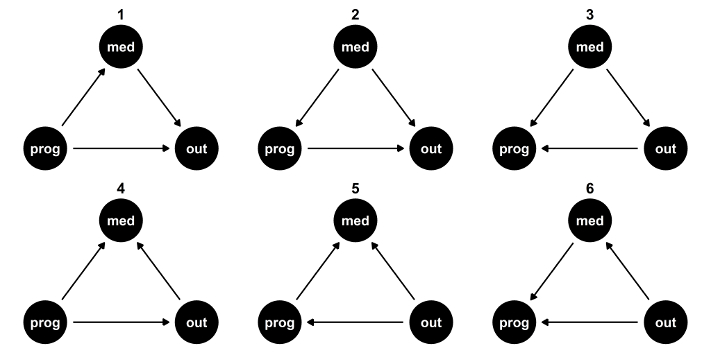
Additionally, a large number of causal models will be consistent with the data, so you need a theory to choose between them. For example, given only data, the following six simple causal models are statistically equivalent. Each model has three variables: outcome (out); condition, e.g., the programme being evaluated or usual practice (prog); and mediator (med).
Model 1 is the intended causal interpretation: the effect of the programme is partially explained by the mediator. Model 2, for example, says that programme and outcome are statistically associated with each other because the supposed mediator is actually a common cause.
The Magenta Book recommends using theory-based evaluation if you can’t find a comparison group (HM Treasury, 2020, p. 47). Annex A (analytical methods for use within an evaluation) locates trials and quasi-experiments outside the theory-based list. I think the Magenta Book is partly responsible for perpetuating Myth 5 in the UK – particularly through invitations to tender that follow the book, which leave evaluators having to play a semantic game to win work. I hope the upcoming revision corrects this (update: it doesn’t), and that it becomes routine practice to commission theory-based trials, quasi-experiments, and mixed methods evaluations, alongside theory-based qualitative impact evaluations and small-n case studies.
6. Theories of change are a kind of diagram
Theories of change are theories – of change. They may be illustrated using a diagram, but there needs to be an explanation, usually using prose, describing how the resources, entities (e.g., people, organisations, laws, etc.), and activities carried out lead to outputs and outcomes. Currently entrenched practices of developing a Theory of Change™ seem to lead people to forget what they learned about theory and theorising at university.
Pawson and Tilley (1997, p. 134) provide neat examples of how to organise theories of change explanations in tables. Tables like these are part of the “realist evaluation” tradition; however, the logic is clearly much more general (see Myth 4):
Context
Mechanism
Outcome
High numbers of prepayment meters, with a high proportion of burglaries involving cash from meters
Removal of cash meters reduces incentive to burgle by decreasing actual or perceived rewards
Reduction in percentage of burglaries involving meter breakage; reduced risk of burglary at dwellings where meters are removed; reduced burglary rate overall
If a client forces you to include only a diagram in a report, plead with them to let you add the actual theory to an Appendix. We’ve been in this situation many times and used this solution once to date – let’s see if the report is published (update: it wasn’t).
7. Evaluations test “treatments”
Well, in a formally defined sense they do; however, not as people usually use the term. We’re not administering drugs – we’re evaluating, e.g., mentoring, approaches to teaching, emotional support. The term “treatment” carries with it medical baggage, which is very different to social programmes. My preference would be to use names that are as close as possible to the conditions. For instance, if we were evaluating ACME Therapy, the conditions would be something like ACME Therapy and usual practice or ACME Therapy and CBT.
The same goes for terms like contamination and dosage. Contamination is usually invoked when making the case for cluster randomisation, referring to the risk that individuals in the control group receive elements of the programme being evaluated too, e.g., students telling each other what they learned working with a mentor. Calling it “contamination” implies something toxic or infectious. A better term may be spillover, diffusion, or cross-group knowledge sharing.
Dosage is typically used to describe how much of a programme someone engages with, e.g., the number of sessions attended or hours of support. People aren’t absorbing a dose, they’re participating, doing activities that are suggested, sharing how they feel with a practitioner. Terms like engagement level, participation intensity, or simply sessions attended might better reflect what’s actually going on.
Using medical language in the context of trials in schools or criminal justice sounds especially creepy – it reminds me of A Clockwork Orange. I have been guilty of using these terms too. Sometimes it’s just too difficult to challenge medicalised tradition when there are pressing deadlines, and causal estimands like average treatment effect on the treated are pervasive in the methods literature (e.g., Cunningham, 2021, Section 4.1.2).
Cook, T. D. (2000). The false choice between theory-based evaluation and experimentation. In A. Petrosino, P. J. Rogers, T. A. Huebner, & T. A. Hacsi (Eds.), New directions in evaluation: Program Theory in Evaluation: Challenges and Opportunities (pp. 27–34). Jossey-Bass.
Fitz-Gibbon, C. T., & Morris, L. L. (1975). Theory-based evaluation. Evaluation Comment, 5(1), 1–4. Reprinted in Fitz-Gibbon, C. T., & Morris, L. L. (1996). Theory-based evaluation. Evaluation Practice, 17(2), 177–184.
Something I’d like to play with when I get the chance:
“optweight contains functions to estimate stable balancing weights that balance covariates up to given thresholds. It solves a convex optimization problem to minimize a function of the weights that captures their variability (or divergence from a set of base weights). This is the method described in Zubizarreta (2015), Källberg and Waernbaum (2023), and Wang and Zubizarreta (2020). optweight extends the method to multi-category, continuous, and multivariate treatments and provides a simple user interface and compatibility with the cobalt package for balance assessment. See vignette("optweight") for a more thorough description of the package’s capabilities.”
Something fun (Słoczyński et al., 2025, p. 3, footnote 1):
“IPT [inverse probability tilting] coincides with Hainmueller’s (2012) entropy balancing estimator when the propensity score is estimated with the logit model”.
(It just holds for ATT.) The picture below illustrates the correspondence, using the Lalonde (1986) dataset (in the cobalt package in R). I computed (knitted R here) the weights using the WeightIt package (Greifer, 2025). Since we’re aiming for ATT, the intervention group weights are all equal to 1, so I’ve omitted them from the graph.
The weights are perfectly correlated and the effective sample sizes are the same. They are scaled differently, though (in the WeightIt implementation at least – need to wade into the original papers): entropy weights sum to the comparison group sample size and IPT weights sum to the intervention group sample size.
References
Greifer, N. (2025). WeightIt: Weighting for Covariate Balance in Observational Studies (version 1.5.0) [R Package].
Słoczyński, T., Uysal, S. D., & Wooldridge, J. M. (2025). Covariate Balancing and the Equivalence of Weighting and Doubly Robust Estimators of Average Treatment Effects. IZA Institute of Labour Economics Discussion Paper, 18147.
Here’s a half‑baked idea, inspired by multiple conversations about randomised controlled trials versus quasi‑experiments at the Australian Evaluation Society 2025 conference.
Outcome measurement databases are now a familiar part of evaluation. One database I frequently use is the Child Outcomes Research Consortium (CORC) Directory of Outcome Measures. The Education Endowment Foundation (EEF) has developed similar resources.
Databases like these make it easier to map theories of change outcomes to measures, and they often include information on psychometric properties such as reliability, and pre‑post correlations, which are handy for informing power calculations.
While outcomes receive this collective attention, quasi‑experimental designs hinge just as much on the quality of their covariates. Pre‑intervention measures of outcomes are especially important, given how highly correlated they tend to be with outcomes. That’s the covariate we get for free once we fix on an outcome, but other characteristics of people and contexts are essential too – often a large number of them.
So, the half‑baked idea is this: evaluation should develop a covariates database, organised by topic area and outcome, to provide evaluators with a shared resource to aid the design of quasi‑experiments. A potential name for this shared resource is the Covariate Commons.
The selection of covariates should always be considered on a case‑by‑case basis, guided by the most likely confounding variables (those that correlate both with who engages with a programme and with outcomes). However, evaluators know that some variables appear repeatedly across studies and sometimes across topic areas (age, gender, social deprivation, to name three).
What do you think? Is there already an example of this for some topics? And who should be responsible for developing and maintaining it?
Quasi-experimentalists will be familiar with King and Nielsen’s (2019) landmark paper, Why Propensity Scores Should Not Be Used for Matching. This specifically critiqued the use of propensity scores for matching; other common uses of propensity scores, such as inverse probability weighting, were not affected. An interesting paper has appeared by Fei Wan (2025) critiquing King and Nielsen’s findings.
Fei Wan’s targets include:
The inappropriateness of using an average pairwise covariate distance between treated and closest comparison match to evaluate PSM. Distances are always nonnegative so can’t take account of positive and negative differences averaging out. It’s already known that two observations with the same propensity score are likely to have different covariate values, but it’s ok if they are random.
King and Nielsen used a cherry-picking approach for model selection, trying 512 different specifications and selecting the one that yields the largest average treatment estimate. This is just poor analysis practice.
Fei Wan recommends machine learning approaches to estimate propensity scores, rather than the common use of logistic regression.
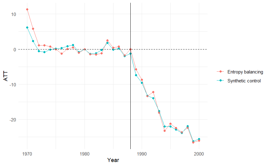
Experimenting with the California tobacco control data used by Abadie, Diamond, and Hainmueller (2010) – here I’m comparing synthetic controls with entropy balancing. The results are remarkably similar, except I had to drop some covariates to get the entropy balancing to find a solution. To be continued…
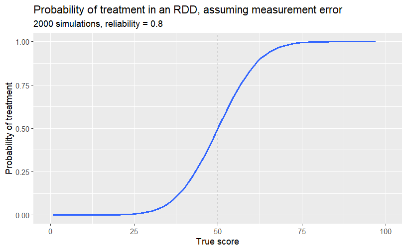
In a sharp regression discontinuity design (RDD), everyone with a running score at or above the threshold gets the treatment and nobody below does. It looks like the propensity of treatment at or above threshold is 1 and below is 0. However, with measurement error, someone’s running score could have been different and near the threshold this could have affected their treatment assignment. This is the genre of justification often seen for why RDDs act like randomised experiments near the threshold.
Under classical test theory,
observed score = true score + error
and a measure’s reliability is
var(true score) / var(observed score).
(We usually don’t see the true score, hence the need for estimators like Cronbach’s α and McDonald’s ω.)
The picture below is from a simulation where we keep people’s true running score fixed (normal distro, mean = 50, SD = 20) but let the observed running score randomly vary due to the unreliability. The probability of treatment is then the proportion of times across simulations that someone ends up in treatment.
So, close to the threshold, the probability of treatment is nearest 50-50.
(I tried and failed to find this pic in the lit; the closest I could spot is in Scott Cunningham’s Mix Tape.)