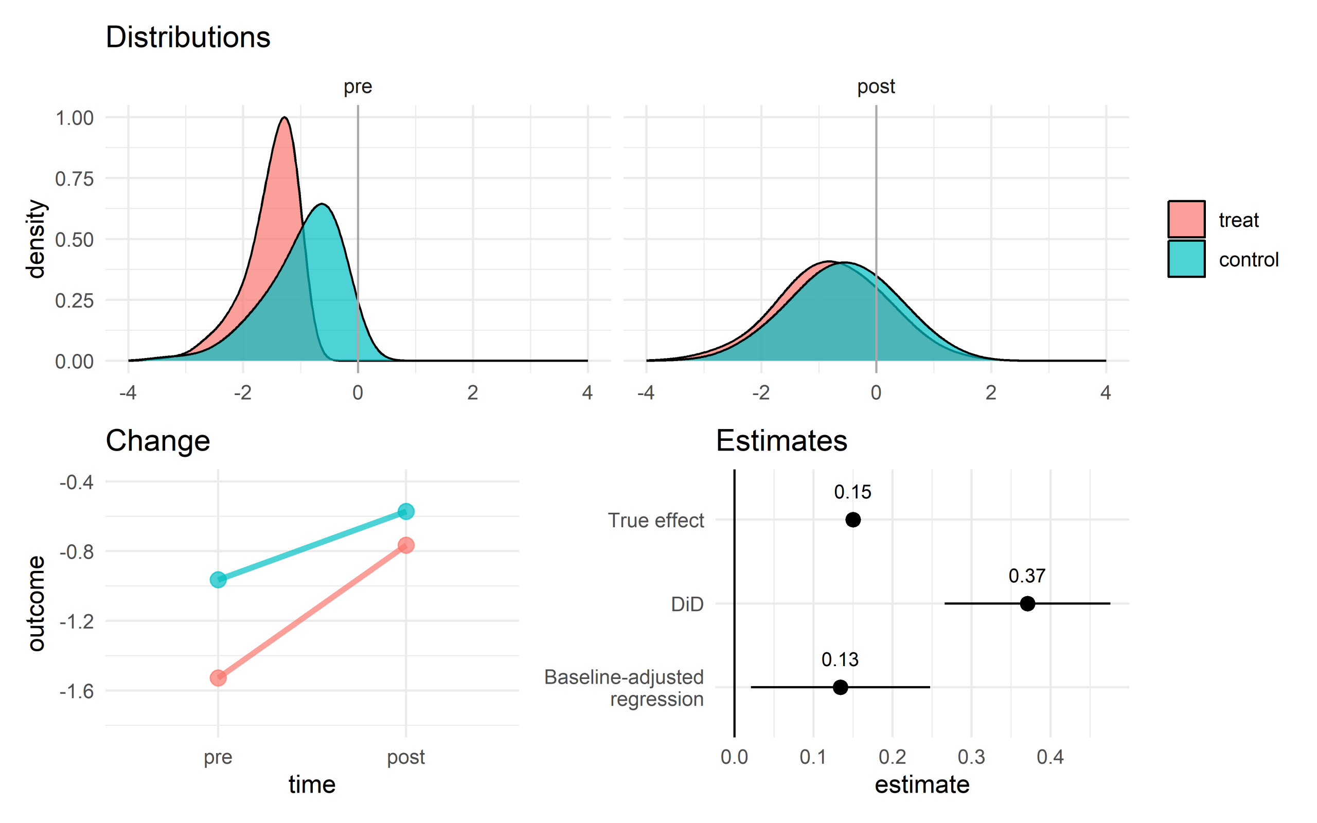
In another episode of, I wonder how well just regressing outcome on intervention group and baseline will do…? Here’s a scenario which breaks the diff-in-diffs parallel trends assumption using regression to the mean.
The treatment group observations were selected so they’re further below the mean at baseline than the control group observations, so by regression to the mean alone, the treat group will show more change. (Pre-post correlation 0.6 in the population, before selection.)
The DiD model was the usual 2×2 approach with participant fixed effects, which control for time-invariant effects that will not save us here.
The baseline-adjusted model regresses outcome on group and baseline.
The only confounder is baseline.
See Ryan (2018) for discussion of some of the muddles in the DiD lit on these kinds of effects.
References
Ryan, A. M. (2018). Well‐Balanced or too Matchy–Matchy? The Controversy over Matching in Difference‐in‐Differences. Health Services Research, 53(6), 4106–4110.
selectTWFE looks interesting: “Estimates both a vanilla two-way fixed effects (TWFE) model and an extended TWFE (ETWFE) model, then selects between them using Cochran’s Q test for heterogeneity. When ETWFE wins, reports the heterogeneity fraction (I-squared) and cohort-time estimates with empirical Bayes shrinkage and Bonferroni multiplicity correction.”
Two papers caught my attention on sample‑size calculation: one for difference‑in‑differences designs (Hedberg & Hedges, 2026) and another for propensity score weighted designs (Liu et al., 2026).
Difference-in-differences (DiD)
Hedberg and Hedges (2026) have developed a method for estimating minimum detectable effect size (MDES) for DiD, including R code in an appendix. The approach takes account of variance explained by covariates (which could include fixed effects for units) and covariate imbalance. It also allows for unequal sample sizes. To run in reverse and estimate sample sizes, there’s a multitude of ways to get R to search across a range of sample sizes and minimise the difference between the achieved and target MDES.
Some things to bear in mind:
It handles both repeated cross-sectional and mixed between-within designs; for the latter, use fixed effects (so \(n-1\) covariates for \(n\) units) alongside an estimate of the variance explained. The parameters include the number of observations, not participants. So for a 2×2 design with pre and post measures from each participant, you will need to multiply the number of participants by 2.
There’s an error in the published code:
if (rho1 > 1) {
  V <- V*(1/(1-rho1^2))
}
if (rho2 > 1) {
  V <- V*(1-rho2^2)
}
Those rhos should never be over 1, and earlier checks won’t allow them to be. The code should check if they are over zero:
if (rho1 > 0) {
  V <- V*(1/(1-rho1^2))
}
if (rho2 > 0) {
  V <- V*(1-rho2^2)
}
I spotted this during testing: increasing the variance explained by covariates did not affect the MDES, and the results differed from the simulation checks. The corrected version resolves this, and the authors very kindly and promptly confirmed the fix. I understand that updated code will be available on the journal’s website soon. In the meantime, the edits noted above should address the issue.
Propensity score weighting
I had been using Austin’s (2021) work to approximate VIFs from c-statistics of propensity score models, which represent lack of overlap in propensity score distributions between groups. The resulting VIFs can then be used to inflate sample sizes estimated from standard power calculators.
Liu, Yang, and Li (2026) have developed an alternative approach that does the sample size estimation in one go, depending on prevalence of the intervention, and an overlap parameter, \(\phi\), which is 1 with perfect overlap and decreases as the propensity score distributions separate. The approach has been implemented in the R package PSpower, which is on CRAN.
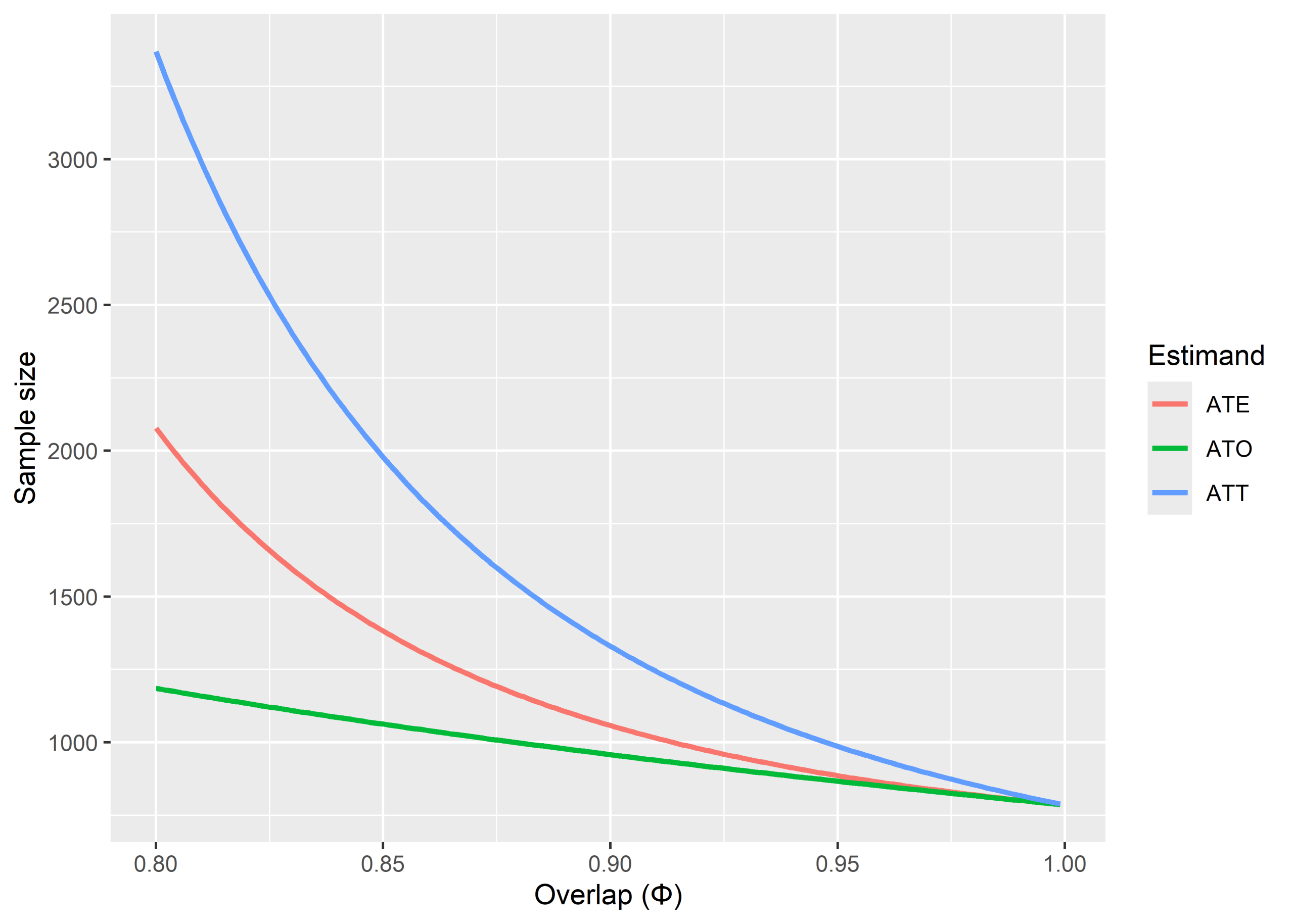
It’s speedy. Here’s an example with intervention prevalence at 50%, MDES 0.2, and varying the overlap from 80% to 99%, for the ATE, ATT, and ATO estimands. ATO is least affected by lack of overlap because it deliberately defines the estimand on the region where there is most overlap and down-weights observations that are far from there. ATO has a policy interpretation too: impact for people in the region of decisional equipoise.
“The starting point of this paper was a 2 × 2 DiD design that researchers have been using for almost 200 years. The end point was a design with five treatment groups, 11 years of data, six covariates, three types of parallel trends assumptions, and four estimation techniques.”
Baker, A., Callaway, B., Cunningham, S., Goodman-Bacon, A., & Sant’Anna, P. H. C. (2025). Difference-in-Differences Designs: A Practitioner’s Guide (No. arXiv:2503.13323). arXiv. https://doi.org/10.48550/arXiv.2503.13323
“I have done a lot of work on difference-in-differences (DiD), and have tried to make as many resources as possible available online. This page collects links to those resources.”
“The man who has fed the chicken every day throughout its life at last wrings its neck instead, showing that more refined views as to the uniformity of nature would have been useful to the chicken.” – Bertrand Russell (1912/2001, p. 35)
The parallel trends assumption of difference-in-differences (diff-in-diffs) is that the average outcomes for intervention and comparison groups would have continued in parallel from pre- to post-intervention if the intervention had not been introduced. This assumption cannot be directly tested, since when diff-in-diffs is used, the intervention is introduced. However, a case is often made that parallel trends probably holds (or doesn’t not hold) by analysing pre-intervention trends.
The mystery graph below shows an example from Kahn-Lang and Lang (2020, p. 618), redrawn to add some suspense:
The averages for the two groups (A and B) are practically identical and remain parallel. I can also reveal that there is a large number of observations – enough to be really confident that the lines are parallel. Given data like this, many of us would be confident that we had found no evidence against parallel trends.
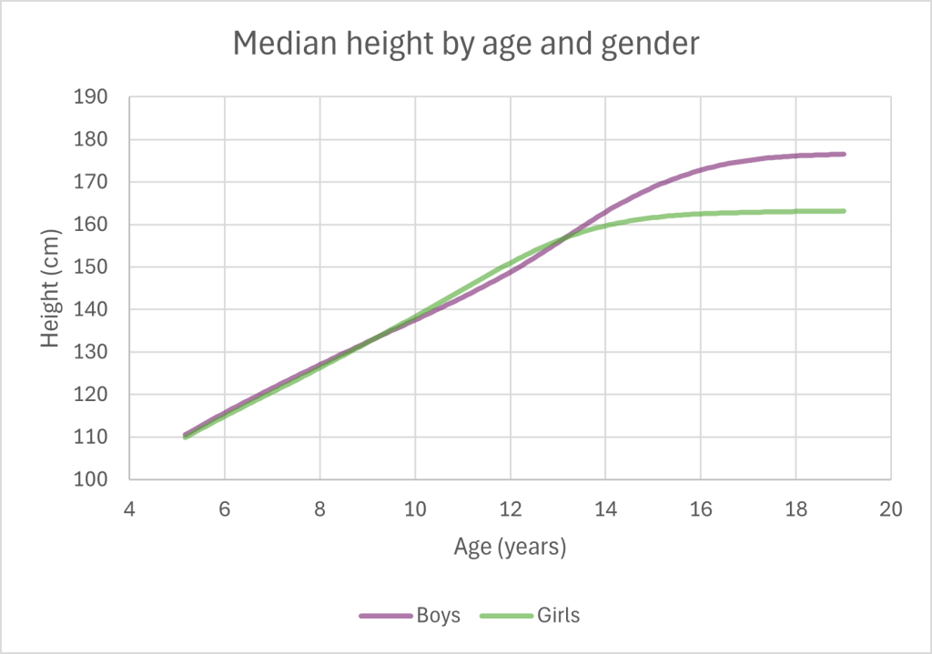
Alas, once the time series is extended, we see that the averages significantly diverge. Adding titles to the graph reveals why – it shows median height by gender from the ages 5 to 19:
Growth reference data from WHO; see percentiles for girls and boys xlsx files over here
Around age 9, the median girls’ height begins to exceed boys’, the difference peaking at about 12 years old. Then the difference in medians decreases until around 13 when boys’ median height begins to exceeds girls’.
Clearly, if we wanted to evaluate, e.g., an intervention to boost children’s height, we wouldn’t compare the mean height of one gender with another as control. The biological processes underpinning gender differences in pubertal growth spurt are well-known. However, diff-in-diffs is often applied in situations where much less is known about how changes occur over time.
As this example illustrates, the more we know about the topic under investigation and the more covariates we have at our disposal for choosing comparison units, the better our causal estimates using diff-in-diffs are likely to be. Diff-in-diffs can also be combined with matching or weighting on covariates to help construct a comparison group such that parallel trends is more likely to hold; see, e.g., Huntington-Klein (2022, Section 18.3.2).