Two papers caught my attention on sample‑size calculation: one for difference‑in‑differences designs (Hedberg & Hedges, 2026) and another for propensity score weighted designs (Liu et al., 2026).
Difference-in-differences (DiD)
Hedberg and Hedges (2026) have developed a method for estimating minimum detectable effect size (MDES) for DiD, including R code in an appendix. The approach takes account of variance explained by covariates (which could include fixed effects for units) and covariate imbalance. It also allows for unequal sample sizes. To run in reverse and estimate sample sizes, there’s a multitude of ways to get R to search across a range of sample sizes and minimise the difference between the achieved and target MDES.
Some things to bear in mind:
It handles both repeated cross-sectional and mixed between-within designs; for the latter, use fixed effects (so \(n-1\) covariates for \(n\) units) alongside an estimate of the variance explained. The parameters include the number of observations, not participants. So for a 2×2 design with pre and post measures from each participant, you will need to multiply the number of participants by 2.
There’s an error in the published code:
if (rho1 > 1) {
  V <- V*(1/(1-rho1^2))
}
if (rho2 > 1) {
  V <- V*(1-rho2^2)
}
Those rhos should never be over 1, and earlier checks won’t allow them to be. The code should check if they are over zero:
if (rho1 > 0) {
  V <- V*(1/(1-rho1^2))
}
if (rho2 > 0) {
  V <- V*(1-rho2^2)
}
I spotted this during testing: increasing the variance explained by covariates did not affect the MDES, and the results differed from the simulation checks. The corrected version resolves this, and the authors very kindly and promptly confirmed the fix. I understand that updated code will be available on the journal’s website soon. In the meantime, the edits noted above should address the issue.
Propensity score weighting
I had been using Austin’s (2021) work to approximate VIFs from c-statistics of propensity score models, which represent lack of overlap in propensity score distributions between groups. The resulting VIFs can then be used to inflate sample sizes estimated from standard power calculators.
Liu, Yang, and Li (2026) have developed an alternative approach that does the sample size estimation in one go, depending on prevalence of the intervention, and an overlap parameter, \(\phi\), which is 1 with perfect overlap and decreases as the propensity score distributions separate. The approach has been implemented in the R package PSpower, which is on CRAN.
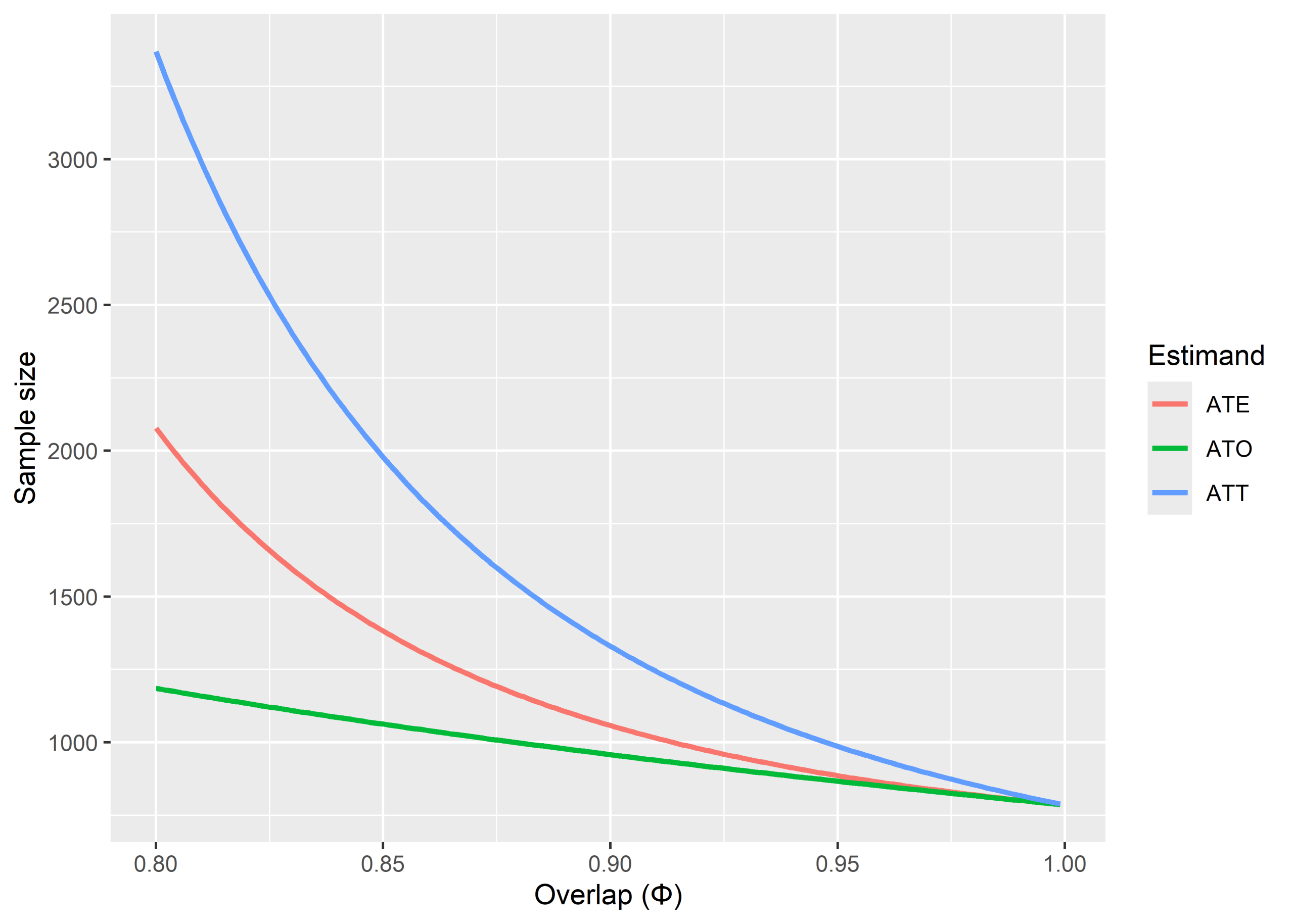
It’s speedy. Here’s an example with intervention prevalence at 50%, MDES 0.2, and varying the overlap from 80% to 99%, for the ATE, ATT, and ATO estimands. ATO is least affected by lack of overlap because it deliberately defines the estimand on the region where there is most overlap and down-weights observations that are far from there. ATO has a policy interpretation too: impact for people in the region of decisional equipoise.
References
Austin, P. C. (2021). Informing power and sample size calculations when using inverse probability of treatment weighting using the propensity score. Statistics in Medicine, 2, 1–14.
Liu, B., Yang, C., & Li, F. (2026). Sample size and power calculations for causal inference of observational studies (Version 5). arXiv, to appear in Annals of Statistics.
Hedberg, E. C., & Hedges, L. V. (2026). Computing Statistical Power for the Difference in Differences Design. Evaluation Review, 50(1), 149–180.
