“Generative” causation

“For the believer in generative causality the existence of the statistics is but the first step in a long process of investigation which ends only when the nature of the things involved has been found out and the reasons for the statistics thus elicited. Science follows the generative rather than the successionist theory of causality.”

– Rom Harré (1972, p. 118)

Harre, R. (1972). The philosophies of science. Oxford University Press.

How p-values are distributed if the null hypothesis is true

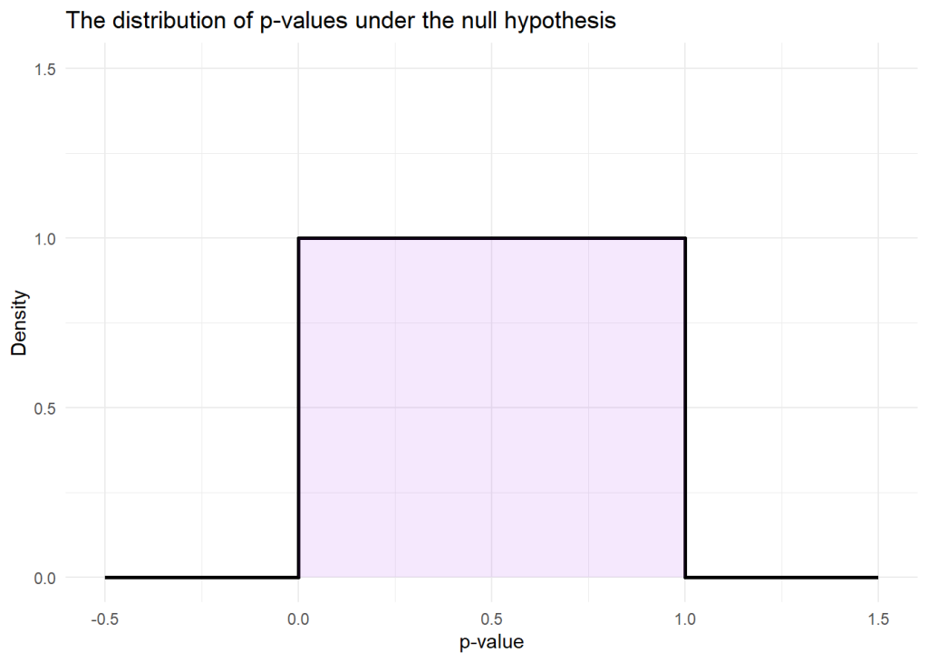
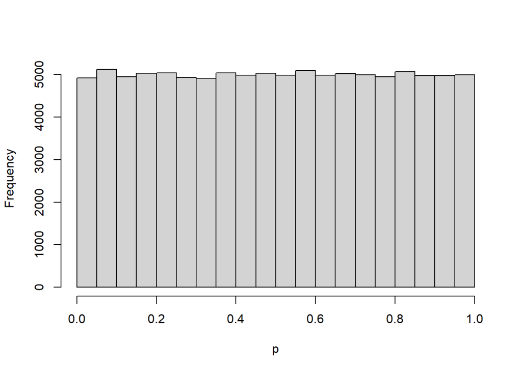
Here’s something random: how p-values are distributed if the null hypothesis is true. It’s the uniform distribution over the unit interval, [0, 1]. So every p-value between 0 and 1 is equally likely if the null hypothesis is true.

Here’s some R code to simulate:

null_distro <- function() {
x <- rnorm(100)
y <- rnorm(100)
t.test(x, y)$p.value
}
replicate(100000, null_distro()) |>
hist(main = "", xlab = "p")

Propensity score analysis with baseline measure of outcome

Mild headache in this new simulation study by Peter Austin of propensity score matching/weighting studies where you have a baseline measurement of the outcome variable – a useful thing to balance as it’s often highly correlated with outcome.

For ATE, the recommendations make sense: include the baseline in the propensity model and then, for what are often called doubly robust approaches, include baseline again as a covariate in the outcome model.

For ATT, the findings are not what I would have expected. Austin’s recommendation for best standard errors is to exclude the baseline from the propensity model and analyse change from baseline in the outcome model 😱:

“… recommendations for the analysis of RCTs with baseline measurements of the follow-up variable do not reflect perfectly what we observed in the context of the analysis of observational studies using propensity score methods. We found that the analysis of change from baseline using a propensity score that excluded the baseline value of the follow-up variable tended to result in the most precise estimates of treatment effect. However, we did observe that, when using weighting, the use of ANCOVA in conjunction with a propensity score model that included the baseline value of the follow-up variable tended to perform well.”

One to read properly to see what’s going on. Would be interested in your thoughts.

References

Austin, P. (2024). Propensity Score Analysis With Baseline and Follow-Up Measurements of the Outcome Variable. Pharmaceutical Statistics. Early view.
Sampling without replacement with specified marginal sampling probabilities

The {sampling} library by Yves Tillé and Alina Matei implements Brewer’s (1975) method – discussed above – as UPbrewer. Tillé’s (2023) review looks interesting too, cataloguing a bunch of incorrect methods and what to use instead.

References

Brewer, K.E.W. (1975), A simple procedure for sampling πpswor. Australian Journal of Statistics, 17, 166-172.

Tillé, Y. (2023). Remarks on some misconceptions about unequal probability sampling without replacement. Computer Science Review, 47, 100533.

Being brave with causal interpretations

One of the fabulous things about evaluation is that we are allowed to (or, rather, required to!) make causal claims from a wide variety of evidence, not only experiments. Causal estimands, defined in terms of potential outcomes, are the norm for quantitative impact evaluations. Causal DAGs are becoming more popular too and one of my favourite tools for thinking through quasi-experimental designs.

Not all fields have it so good.

Julia Rohrer has written a great blog post, following a series of journal papers, urging personality psychologists to be upfront with their causal claims. It’s challenging to persuade and I think interesting as a sociology of science case study. As Rohrer summarises, ‘Being vague about the desired interpretation may maintain some degree of plausible deniability and potentially offload the error to others (“oh, you shouldn’t have interpreted our numbers like that!1”). But honestly, that’s just a cowardly way to do science. Life is too short for that.’

Comparing {eefAnalytics} and {lmeInfo}

In multilevel analyses, it is often necessary to estimate a standardised mean difference (SMD) where the numerator is a covariate-adjusted mean difference and the denominator is the SD from a model without covariate adjustment.

I’m aware of two (frequentist, non-bootstrap) packages calculating an SMD and confidence interval in R. Here’s a comparison of them for simulated data.

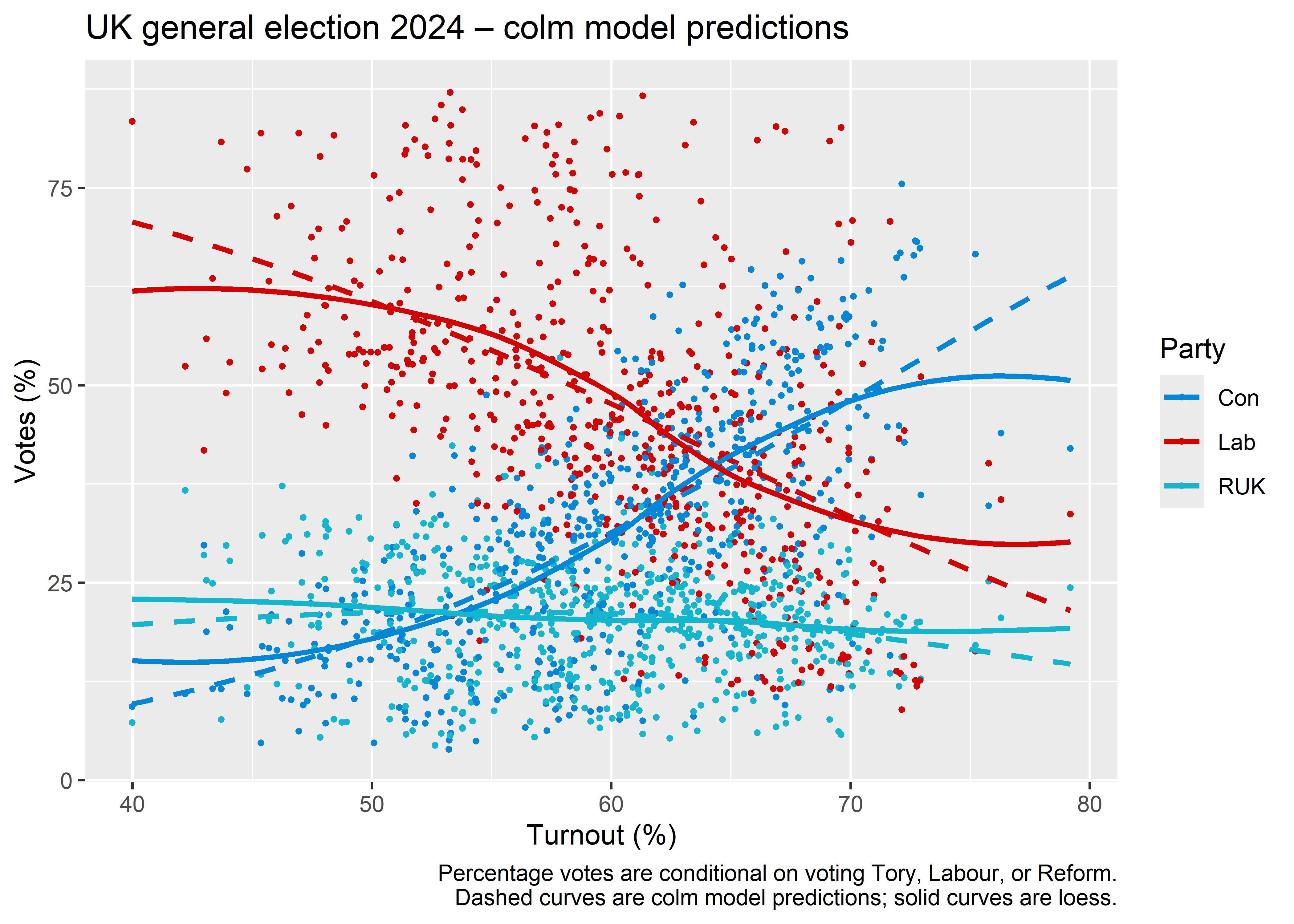
Was turnout associated with the composition of Labour, Tory, and Reform votes?

Was turnout associated with the composition of Labour, Tory, and Reform votes? An excuse to test drive the {compos} package, by David Firth and Fiona Sammut, which implements the generalized Wedderburn logit model. See preprint by Firth and Sammut (2023), Analysis of composition on the original scale of measurement.

Knitted output over here.