One of the fab things about statistics and siblings like psychometrics is that they develop ways to estimate quantities that it is impossible to measure directly, alongside the uncertainty around those estimates. Measure reliability is an example: it tells us how much of the variation in observed scores (e.g., from school exams or mental health symptom measures) is due to actual differences between people in what’s being measured, rather than random error. In classical test theory, reliability (call it \(r\)) is defined as the proportion of observed score variance that reflects true score variance:
\(\displaystyle r = \frac{\sigma^2_T}{\sigma^2_X}\),
where \(\sigma^2_T\) is the variance of the true scores (what we’d see if we could measure perfectly) and \(\sigma^2_X\) is the variance of the scores we actually observe, which includes both true variation and variance due to random error. Making that explicit:
\(\displaystyle r = \frac{\sigma^2_T}{\sigma^2_T + \sigma^2_\epsilon}\),
where \(\sigma^2_\epsilon\) is the error variance. So if \(\sigma^2_\epsilon\) were zero, the reliability would be 1.
Alas, we can’t directly observe the true scores, so we can’t calculate \(\sigma^2_T\) exactly and can’t calculate reliability. Instead, we estimate reliability using correlations between repeated measurements over time, across items, or between raters.
If you take 30 draws from a Bernoulli distribution, e.g., to randomise people to one of two conditions, there’s a \(\frac{2}{2^{30}} = \frac{1}{2^{29}} = \frac{1}{536,870,912}\) chance that all 30 will be assigned to the same condition (all 1s or all 0s).
That’s vanishingly unlikely, but using the following seed with R’s rbinom produces 30 ones:
Unlikely but possible – even if your random numbers come from atmospheric noise or quantum measurements rather than a pseudorandom generator. If you want to rule out this outcome entirely (make the probability zero), then you don’t actually want independent Bernoulli draws. You’d need a different randomisation scheme, such as blocked randomisation.
I often see reports describing checks on random sequences after they’ve been generated, when the researchers could have saved themselves the effort by building in the kind of randomness they wanted from the start.
P.S. The longest initial runs I know about are for seed 796110494, which yields 31 zeros, and 1002755089, which yields 32 ones.
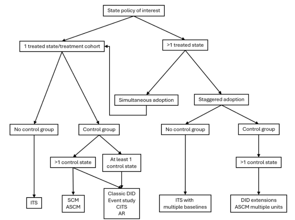
A new preprint by Elizabeth Stone and colleagues explores methods for evaluating state-level policies in the US, offering insights relevant to UK policy evaluation. It covers selection of a range of approaches based on, for example, how a policy varies across the country, whether there is staggered roll out, and the availability of baseline data.
“The starting point of this paper was a 2 × 2 DiD design that researchers have been using for almost 200 years. The end point was a design with five treatment groups, 11 years of data, six covariates, three types of parallel trends assumptions, and four estimation techniques.”
Baker, A., Callaway, B., Cunningham, S., Goodman-Bacon, A., & Sant’Anna, P. H. C. (2025). Difference-in-Differences Designs: A Practitioner’s Guide (No. arXiv:2503.13323). arXiv. https://doi.org/10.48550/arXiv.2503.13323
The Five Safes could be a good way to help think about making data available to “turbocharge” AI [1, 2]. Maybe they already are – but the comms needs to accelerate if so.
Safe projects: Is the proposed use of the data (e.g., ethically) appropriate?
Safe people: Can the analysts be trusted to use it in an appropriate manner? Accredited Researcher registers that many of know and love might help.
Safe data: Is there a disclosure risk in the data itself?
Safe settings: Does the access facility limit unauthorised use? Interesting for cloud-based compute.
Safe outputs: Are the statistical results non-disclosive? This will be particularly challenging for models with millions of parameters.
These are five dimensions and they all need to be considered together to determine whether an approach to making data available is safe. For example if it’s impossible to entirely anonymise data, then the other dimensions need to be beefed up.
[1] Prime Minister sets out blueprint to turbocharge AI. Department for Science, Innovation and Technology, Prime Minister’s Office, 10 Downing Street, The Rt Hon Peter Kyle MP, The Rt Hon Sir Keir Starmer KCB KC MP and The Rt Hon Rachel Reeves MP (13 Jan 2025)
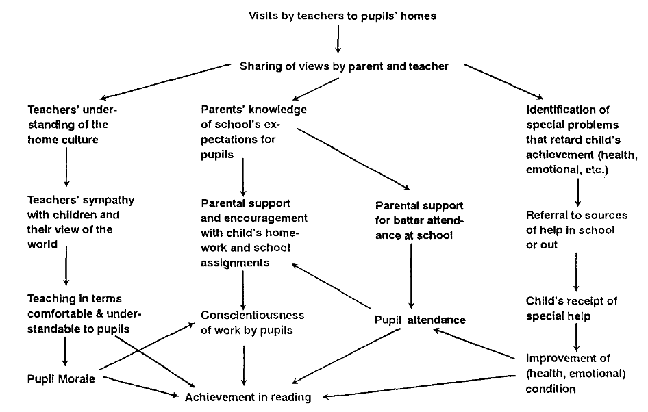
Periodically I listen to contemporary debates in evaluation and wonder how much progress there has been in the past fifty years. Here’s a picture from Carol Weiss (1972, Figure 3–3, p. 50; reprinted in 1996):
Weiss called it a model of a programme; now we would use the term programme theory or theory of change. About half of the next page (Weiss, 1972, p. 51) is filled with intriguing footnotes. The first notes the similarity between the diagram above and a statistical approach:
“As the similarity between Figure 3–3 and a path diagram suggests, path analysis is a useful way of estimating the strength of the linkages. When the necessary conditions for each path analysis are met, path coefficients will represent the magnitude of effects for each arrow.”
On path analysis, Weiss cites Blalock’s (1969) Theory construction from verbal to mathematical formulations. Structural equation modelling, path analysis plus confirmatory factor analysis, turned out to be a popular way to test theories in social science (see, e.g., MacCallum & Austin, 2000; Zyphur, Bonner, & Tay, 2023).
The same footnote also summarises the Automatic Interaction Detector (AID), an early example of a data-driven partitioning procedure:
“Another analytic device, particularly useful when one step in the chain is totally or largely conditional on the one before, is the Automatic Interaction Detector (AID). Unlike path analysis, this type of ‘branch’ analysis shows whether the program is producing strong effects for subsamples of the group. This is a matter of both theoretical and programmatic interest, because if there are differential effects, special programs can be developed to fit special groups.”
AID and its successors are data hungry and liable to overfitting data if misused; however, there is a rich literature on how to use them and stay out of trouble. Loh (2014) reviews fifty years of that literature, beginning with AID (p. 330):
“Despite their novelty, or perhaps owing to it, AID and THAID did not initially attract much interest in the statistics community. Einhorn (1972) showed by simulation that AID can severely overfit the data. Doyle (1973) pointed out that if two or more variables are highly correlated, at most one may appear in the tree structure. This problem of masking can lead to spurious conclusions about the relative importance of the variables. Bishop et al. (1975) criticized AID for ignoring the inherent sampling variability of the data. Around the same time though, the idea of recursive partitioning was gaining steam in the computer science and engineering communities as more efficient algorithms for carrying out the search for splits began to appear (Chou 1969; Henrichon & Fu, 1973; Meisel & Michalopoulos, 1977; Payne & Meisel, 1977; Sethi & Chatterjee, 1991).”
(Example newer algorithms are implemented in {rpart} in R.) Weiss’s footnote and these statistical approaches are clear examples of trying to tackle the “what works best for whom” problem, which for some reason (along with “context”) is now associated, like a Pavlovian response, with “realist” evaluation. We need to do better.
References
Blalock, H. M., Jr. (1969). Theory construction from verbal to mathematical formulations. Prentice-Hall Inc.
MacCallum, R. C., & Austin, J. T. (2000). Applications of structural equation modeling in psychological research. Annual Review of Psychology, 51(1), 201-226.
Weiss, C. H. (1972). Evaluation research: Methods of assessing program effectiveness. Prentice-Hall, Inc.
Weiss, C. H. (1996). Excerpts from evaluation research: Methods of assessing program effectiveness. Evaluation Practice, 17(2), 173–175.
Zyphur, M. J., Bonner, C. V., & Tay, L. (2023). Structural equation modeling in organizational research: The state of our science and some proposals for its future. Annual Review of Organizational Psychology and Organizational Behavior, 10(1), 495-517.
Zimmer, S. A., Powell, R. J., & Velásquez, I. C. (2024). Exploring Complex Survey Data Analysis Using R: A Tidy Introduction with {srvyr} and {survey}. Chapman & Hall: CRC Press.
“The parameters of a statistical model can sometimes be difficult to interpret substantively, especially when that model includes nonlinear components, interactions, or transformations. Analysts who fit such complex models often seek to transform raw parameter estimates into quantities that are easier for domain experts and stakeholders to understand. This article presents a simple conceptual framework to describe a vast array of such quantities of interest, which are reported under imprecise and inconsistent terminology across disciplines: predictions, marginal predictions, marginal means, marginal effects, conditional effects, slopes, contrasts, risk ratios, etc. We introduce marginaleffects, a package for R and Python which offers a simple and powerful interface to compute all of those quantities, and to conduct (non-)linear hypothesis and equivalence tests on them. marginaleffects is lightweight; extensible; it works well in combination with other R and Python packages; and it supports over 100 classes of models, including linear, generalized linear, generalized additive, mixed effects, Bayesian, and several machine learning models.”