Blog post by Andrea Onofri, using {emmeans}, comparing Tukey’s HSD with the multivariate t. Code replicated here.
Lots of useful vignettes on the package page, including for interactions, LMMs, and svyglm.
Personal website – any views expressed herein are my own unless otherwise obvious
Blog post by Andrea Onofri, using {emmeans}, comparing Tukey’s HSD with the multivariate t. Code replicated here.
Lots of useful vignettes on the package page, including for interactions, LMMs, and svyglm.
Looks useful
Data and code from the 2025 paper by Andrew Baker, Brantly Callaway, Scott Cunningham, Andrew Goodman-Bacon, and Pedro H. C. Sant’Anna.
I’m doing Advent of Code again. My answers thus far are on GitHub. I’m aiming for algorithms with worst case time complexity \(\mathcal{O}(\textit{finishes by Christmas})\).

“… the svyglm variance estimator generalises the familiar sandwich estimators to allow for non-trivial sampling.”
Thomas Lumley’s post.
Take \(n\) draws from the uniform distribution on \([0, 1]\), giving \(U_1, U_2, \ldots U_n\).
Iterate \(k\) times, so you end up with a \(k \times n\) matrix.
\(\displaystyle \begin{bmatrix}
U_{1,1} & U_{1,2} & \cdots & U_{1,n} \\
U_{2,1} & U_{2,2} & \cdots & U_{2,n} \\
\vdots & \vdots & \ddots & \vdots \\
U_{k,1} & U_{k,2} & \cdots & U_{k,n}
\end{bmatrix}\)
Then average across those iterations, i.e., average each column, giving \(n\) averages. This gives you the Bates distribution, named after Grace Bates (13 August 1914 – 19 November 1996).
Here’s a picture for six success steps:
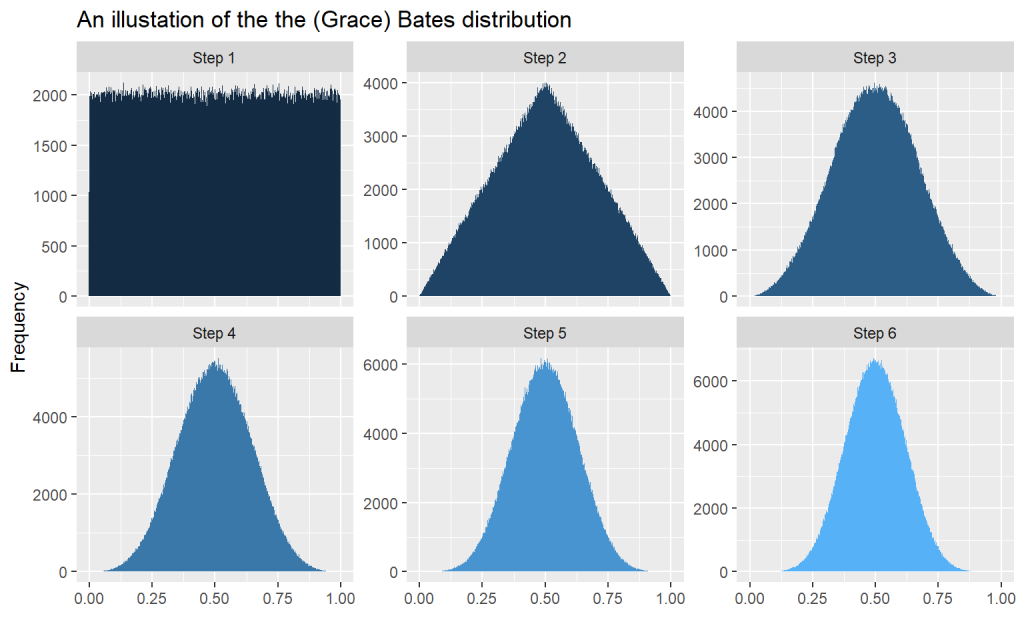
The variance of this is \(\frac{1}{12k}\), which just looks magically simple.
Any Mersenne Twister algorithm experts out there? Based on some experiments, I suspect that the longest initial run of identical values, that is all 0s or all 1s, from rbinom in R is 32. Since that’s a power of 2, I wonder whether it’s an artifact of the algorithm or implementation. Does anyone know?
Here are two seeds I found:
> set.seed(1002755089)
> rbinom(n = 40, size = 1, prob = 0.5)
 [1] 1 1 1 1 1 1 1 1 1 1 1 1 1 1 1 1 1 1 1 1 1 1 1 1 1 1 1 1 1 1 1 1 0 0 1 1 0 0 1 1

> set.seed(-1144728559)
> rbinom(n = 40, size = 1, prob = 0.5)
 [1] 0 0 0 0 0 0 0 0 0 0 0 0 0 0 0 0 0 0 0 0 0 0 0 0 0 0 0 0 0 0 0 0 1 1 0 0 1 1 0 0
Edited (9 Nov 2025) to add: one working hypothesis is that the number of initial runs is driven by the seed space (\(2^{32}\) integers) and the probability of runs over that – so constrained by probability rather than the algorithm. Jan van der Laan (@dodecadron@datasci.social) looked for runs in a long vector of rbinom draws on a fixed seed and found one length 33 further along the sequence (somewhere).
set.seed(182) > x <- rbinom(1e8, 1, 0.5)
r <- rle(x)
table(r$lengths)
If you take 30 draws from a Bernoulli distribution, e.g., to randomise people to one of two conditions, there’s a \(\frac{2}{2^{30}} = \frac{1}{2^{29}} = \frac{1}{536,870,912}\) chance that all 30 will be assigned to the same condition (all 1s or all 0s).
That’s vanishingly unlikely, but using the following seed with R’s rbinom produces 30 ones:
> set.seed(236903047)
> rbinom(30, size = 1, prob = 0.5)
[1] 1 1 1 1 1 1 1 1 1 1 1 1 1 1 1 1 1 1 1 1 1 1 1 1 1 1 1 1 1 1
The seed below produces 30 zeros:
> set.seed(627034302)
> rbinom(30, size = 1, prob = 0.5)
[1] 0 0 0 0 0 0 0 0 0 0 0 0 0 0 0 0 0 0 0 0 0 0 0 0 0 0 0 0 0 0
Unlikely but possible – even if your random numbers come from atmospheric noise or quantum measurements rather than a pseudorandom generator. If you want to rule out this outcome entirely (make the probability zero), then you don’t actually want independent Bernoulli draws. You’d need a different randomisation scheme, such as blocked randomisation.
I often see reports describing checks on random sequences after they’ve been generated, when the researchers could have saved themselves the effort by building in the kind of randomness they wanted from the start.
P.S. The longest initial runs I know about are for seed 796110494, which yields 31 zeros, and 1002755089, which yields 32 ones.
Something I’d like to play with when I get the chance:
“optweight contains functions to estimate stable balancing weights that balance covariates up to given thresholds. It solves a convex optimization problem to minimize a function of the weights that captures their variability (or divergence from a set of base weights). This is the method described in Zubizarreta (2015), Källberg and Waernbaum (2023), and Wang and Zubizarreta (2020). optweight extends the method to multi-category, continuous, and multivariate treatments and provides a simple user interface and compatibility with the cobalt package for balance assessment. See vignette("optweight") for a more thorough description of the package’s capabilities.”
Something fun (Słoczyński et al., 2025, p. 3, footnote 1):
“IPT [inverse probability tilting] coincides with Hainmueller’s (2012) entropy balancing estimator when the propensity score is estimated with the logit model”.
(It just holds for ATT.) The picture below illustrates the correspondence, using the Lalonde (1986) dataset (in the cobalt package in R). I computed (knitted R here) the weights using the WeightIt package (Greifer, 2025). Since we’re aiming for ATT, the intervention group weights are all equal to 1, so I’ve omitted them from the graph.

The weights are perfectly correlated and the effective sample sizes are the same. They are scaled differently, though (in the WeightIt implementation at least – need to wade into the original papers): entropy weights sum to the comparison group sample size and IPT weights sum to the intervention group sample size.
Greifer, N. (2025). WeightIt: Weighting for Covariate Balance in Observational Studies (version 1.5.0) [R Package].
Słoczyński, T., Uysal, S. D., & Wooldridge, J. M. (2025). Covariate Balancing and the Equivalence of Weighting and Doubly Robust Estimators of Average Treatment Effects. IZA Institute of Labour Economics Discussion Paper, 18147.