Intention to treat (ITT) analyses code a participant’s group according to the condition they were assigned to, regardless of whether they engaged with that condition or, e.g., swapped to another. Sometimes the average treatment effect on the treated (ATT) estimand is misunderstood to mean analysing people according to what intervention they actually engaged with. But the two concepts are independent of each other and depend on how the potential outcomes are defined.
For example, let Yᵢ(ai) denote the potential outcome for participant, i, were they to be assigned to the intervention, and Yᵢ(ac) denote the potential outcome were they to be assigned to some comparison condition. Let Gᵢ denote the group they were assigned to (note, not necessarily what they engaged with!). The following estimand is an ITT ATT:
E[Yᵢ(ai) – Yᵢ(ac) | Gᵢ = ai]
Tag: quasi-experiments
Key study design considerations in state policy evaluation
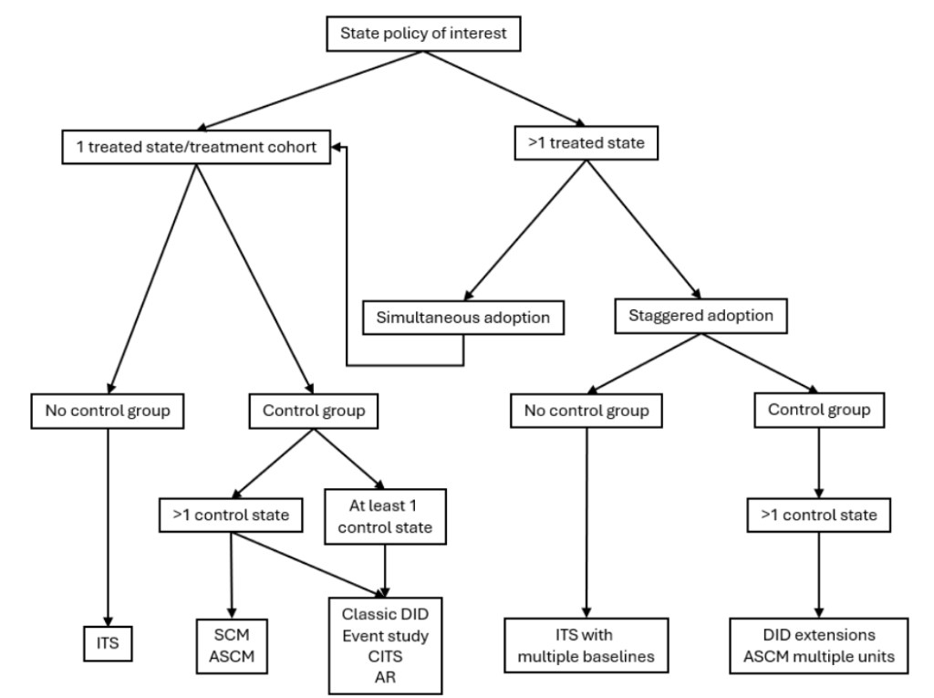
A new preprint by Elizabeth Stone and colleagues explores methods for evaluating state-level policies in the US, offering insights relevant to UK policy evaluation. It covers selection of a range of approaches based on, for example, how a policy varies across the country, whether there is staggered roll out, and the availability of baseline data.
References
Stone, E. M., Schuler, M. S., Stuart, E. A., Rubinstein, M., Griswold, M., Stein, B. D., & Griffin, B. A. (2025). Choosing an analytic approach: Key study design considerations in state policy evaluation.
New review of approaches to adjusting for observed confounders
Just out in Statistics in Medicine, this is a helpful review of approaches to adjusting for observed confounding in non-randomised evaluations (and other studies). Includes a concise summary of assumptions, using the Neyman–Rubin potential outcomes framework.
Keele, L., & Grieve, R. (2025). So Many Choices: A Guide to Selecting Among Methods to Adjust for Observed Confounders. Statistics in Medicine, 44(5), e10336.
Carefully controlled nonrandomised studies give us subjective randomisation
“Consider a carefully controlled nonrandomized study – a study in which there are no obviously important prior variables that systematically differ in the E trials and the C trials. In such a study, there is a real sense in which a claim of ‘subjective randomization’ can be made. For example, if the study was composed of carefully matched pairs of trials, there might be a very defensible belief that within each matched pair each unit was equally likely to receive E as C in the sense that if you were shown the units without being told which received E, only half the time would you correctly guess which received E.”
Rubin, D. B. (1974, p. 698). Estimating causal effects of treatments in randomized and nonrandomized studies. Journal of Educational Psychology, 66(5), 688–701.
See also:
“Matching can be thought of as a technique for finding approximately ideal experimental data hidden within an observational data set.”
King, G., & Nielsen, R. (2019, p. 442). Why Propensity Scores Should Not Be Used for Matching. Political Analysis, 27(4), 435–454.
Pedro Sant’Anna’s materials on difference-in-differences
Mixtape sessions
Lots of readings, slides, and Shiny apps over here.
A contrived example to break diff-in-diffs
Using my favourite tricks to setup the simulation:
- Measurement error
- Select people who are far from the mean
- Ensure there is no true change
Knitted R over here.
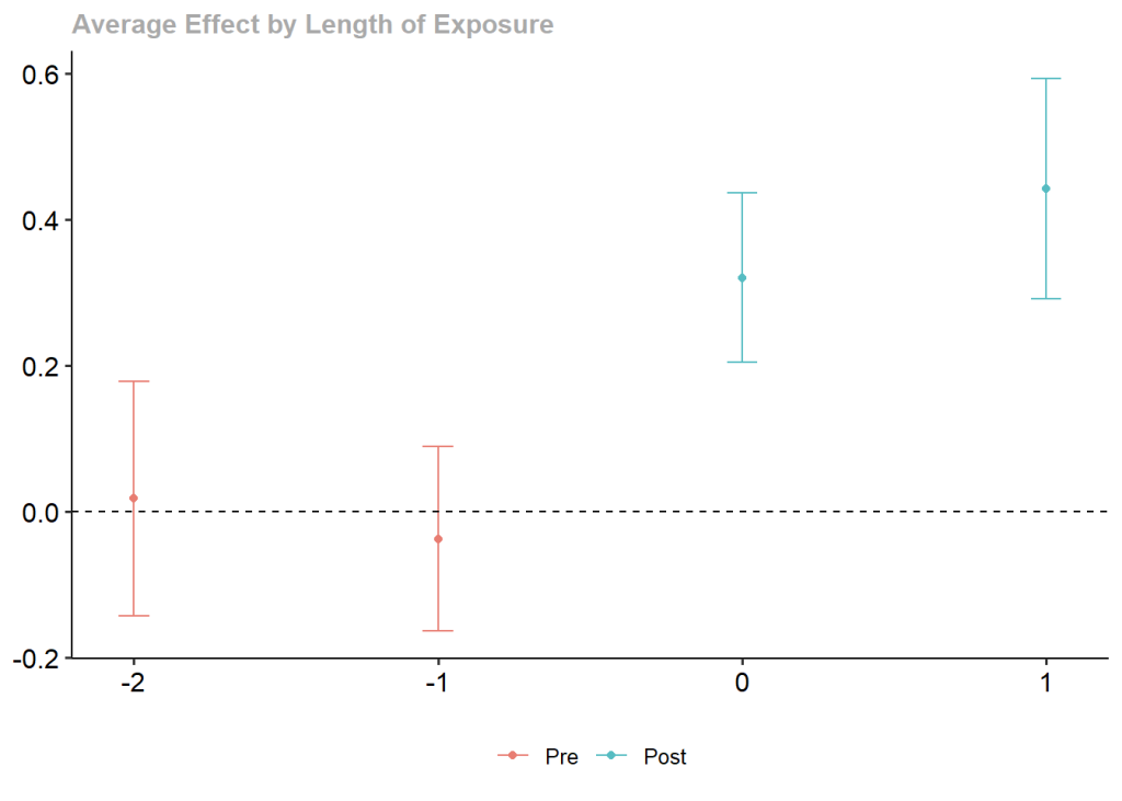
This plot provides some clues (group 0 is never treated; group 3 treated at time 3 and group 4 at time 4):
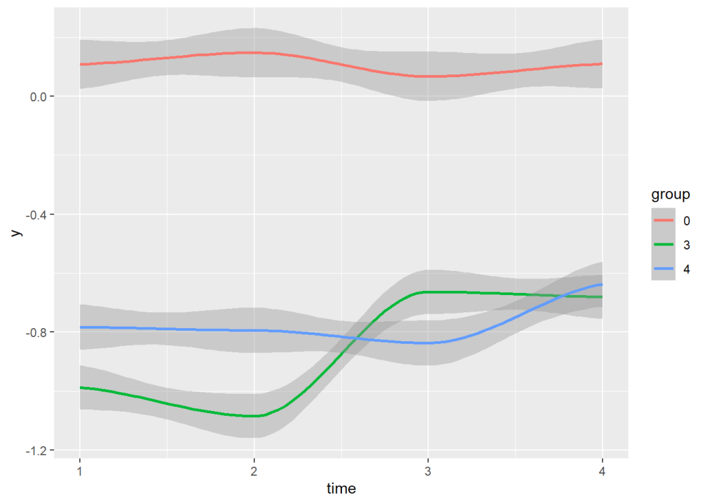
Replicating Callaway and Sant’Anna (2021)
Part 1: ATT(g, t) estimates and pooling across groups. Standard errors coming later.
Chocolate and diabetes
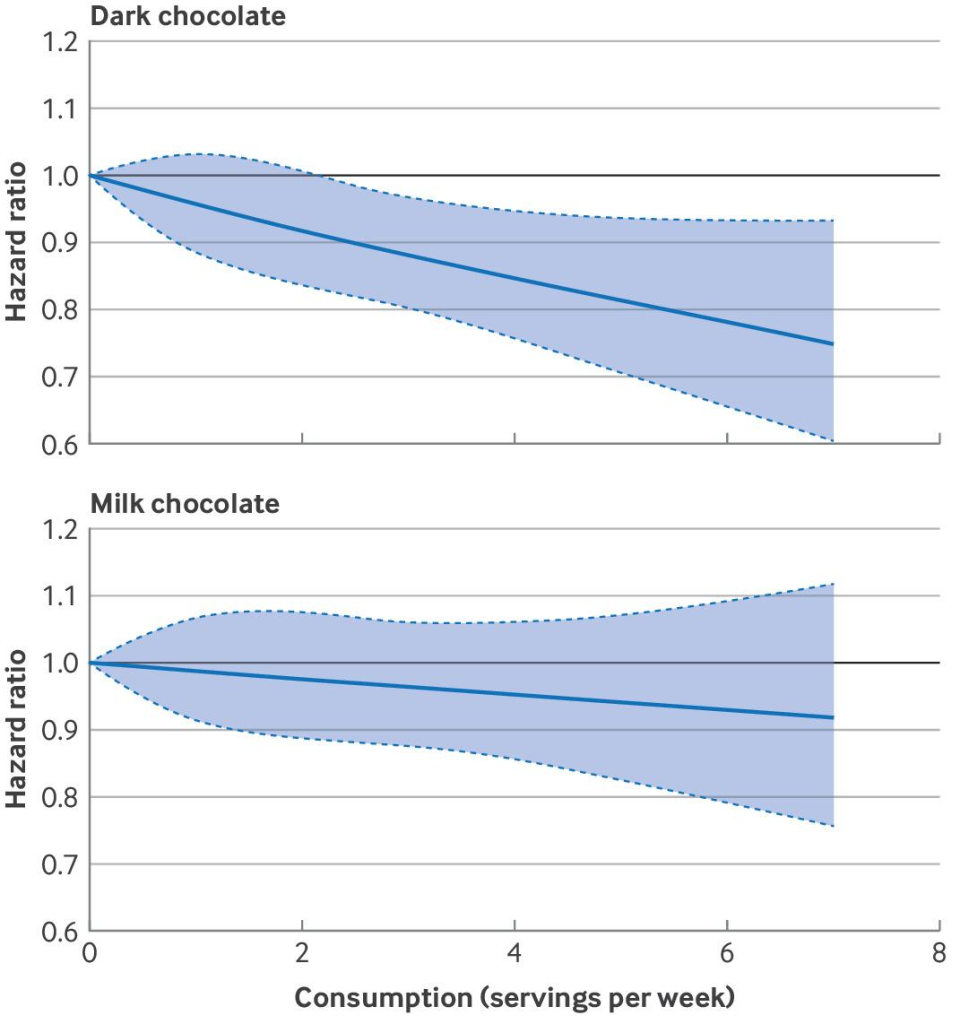
Increased consumption of dark, but not milk, chocolate was “associated with” lower risk of type 2 diabetes (Lin, et al., 2024). Refresh your teaching examples for causal inference using non-experimental data 🤓
Liu, B., Zong, G., Zhu, L., Hu, Y., Manson, J. E., Wang, M., Rimm, E. B., Hu, F. B., & Sun, Q. (2024). Chocolate intake and risk of type 2 diabetes: prospective cohort studies. BMJ, e078386.
Propensity score analysis with baseline measure of outcome
Mild headache in this new simulation study by Peter Austin of propensity score matching/weighting studies where you have a baseline measurement of the outcome variable – a useful thing to balance as it’s often highly correlated with outcome.
For ATE, the recommendations make sense: include the baseline in the propensity model and then, for what are often called doubly robust approaches, include baseline again as a covariate in the outcome model.
For ATT, the findings are not what I would have expected. Austin’s recommendation for best standard errors is to exclude the baseline from the propensity model and analyse change from baseline in the outcome model 😱:
“… recommendations for the analysis of RCTs with baseline measurements of the follow-up variable do not reflect perfectly what we observed in the context of the analysis of observational studies using propensity score methods. We found that the analysis of change from baseline using a propensity score that excluded the baseline value of the follow-up variable tended to result in the most precise estimates of treatment effect. However, we did observe that, when using weighting, the use of ANCOVA in conjunction with a propensity score model that included the baseline value of the follow-up variable tended to perform well.”
One to read properly to see what’s going on. Would be interested in your thoughts.
References
Austin, P. (2024). Propensity Score Analysis With Baseline and Follow-Up Measurements of the Outcome Variable. Pharmaceutical Statistics. Early view.