“I have done a lot of work on difference-in-differences (DiD), and have tried to make as many resources as possible available online. This page collects links to those resources.”
Tag: quasi-experiments
LaLonde (1986) after Nearly Four Decades: Lessons Learned (Guido Imbens, Yiqing Xu)
“We show that modern methods, when applied in contexts with significant covariate overlap, yield robust estimates for the adjusted differences between the treatment and control groups. However, this does not mean that these estimates are valid. To assess their credibility, validation exercises (such as placebo tests) are essential, whereas goodness of fit tests alone are inadequate. Our findings highlight the importance of closely examining the assignment process, carefully inspecting overlap, and conducting validation exercises when analyzing causal effects with nonexperimental data.”
On the parallel trends assumption in difference-in-differences (diff-in-diffs)
“The man who has fed the chicken every day throughout its life at last wrings its neck instead, showing that more refined views as to the uniformity of nature would have been useful to the chicken.”
– Bertrand Russell (1912/2001, p. 35)
The parallel trends assumption of difference-in-differences (diff-in-diffs) is that the average outcomes for intervention and comparison groups would have continued in parallel from pre- to post-intervention if the intervention had not been introduced. This assumption cannot be directly tested, since when diff-in-diffs is used, the intervention is introduced. However, a case is often made that parallel trends probably holds (or doesn’t not hold) by analysing pre-intervention trends.
The mystery graph below shows an example from Kahn-Lang and Lang (2020, p. 618), redrawn to add some suspense:

The averages for the two groups (A and B) are practically identical and remain parallel. I can also reveal that there is a large number of observations – enough to be really confident that the lines are parallel. Given data like this, many of us would be confident that we had found no evidence against parallel trends.
Alas, once the time series is extended, we see that the averages significantly diverge. Adding titles to the graph reveals why – it shows median height by gender from the ages 5 to 19:
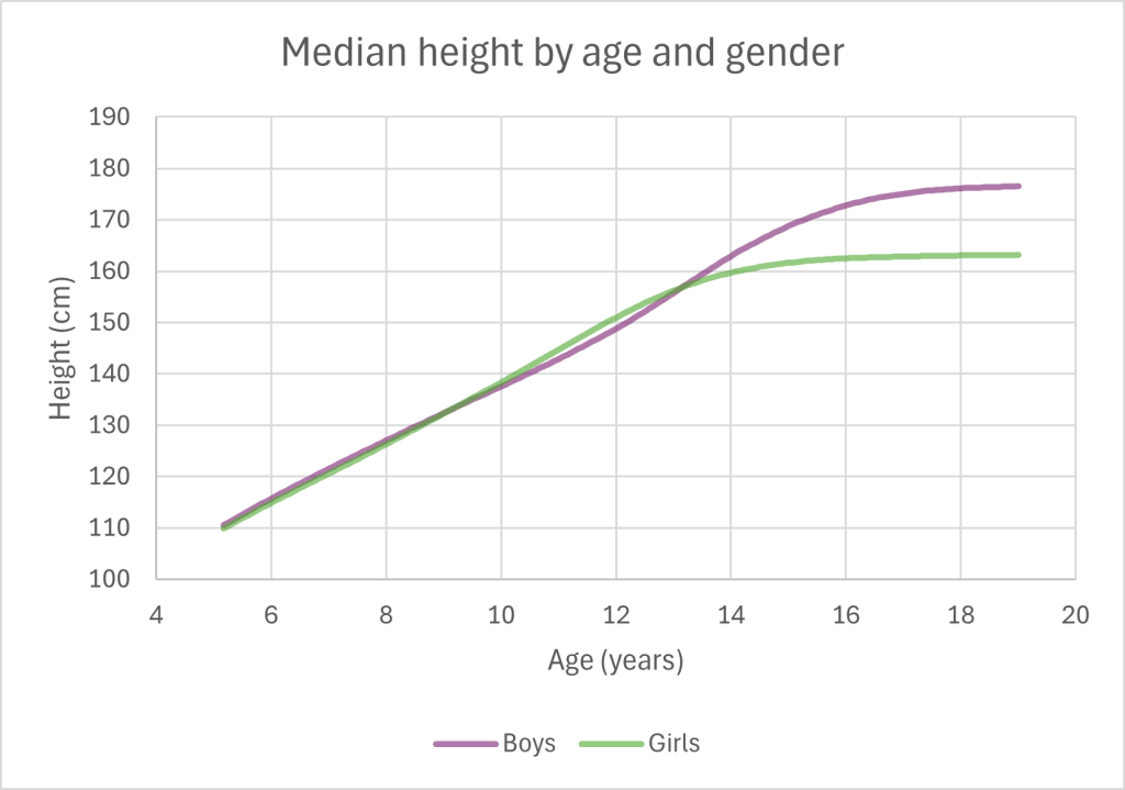
Around age 9, the median girls’ height begins to exceed boys’, the difference peaking at about 12 years old. Then the difference in medians decreases until around 13 when boys’ median height begins to exceeds girls’.
Clearly, if we wanted to evaluate, e.g., an intervention to boost children’s height, we wouldn’t compare the mean height of one gender with another as control. The biological processes underpinning gender differences in pubertal growth spurt are well-known. However, diff-in-diffs is often applied in situations where much less is known about how changes occur over time.
As this example illustrates, the more we know about the topic under investigation and the more covariates we have at our disposal for choosing comparison units, the better our causal estimates using diff-in-diffs are likely to be. Diff-in-diffs can also be combined with matching or weighting on covariates to help construct a comparison group such that parallel trends is more likely to hold; see, e.g., Huntington-Klein (2022, Section 18.3.2).
References
Huntington-Klein, N. (2022). The effect: An introduction to research design and causality. CRC Press.
Kahn-Lang, A., & Lang, K. (2020). The Promise and Pitfalls of Differences-in-Differences: Reflections on 16 and Pregnant and Other Applications. Journal of Business & Economic Statistics, 38(3), 613–620.
Russell, B. (1912/2001). The problems of philosophy. Oxford University Press.
TBE QEDs
‘In TBE [theory-based evaluation] practice […] theory as represented is not specific enough to support causal conclusions in inference […]. For example, in contribution analysis “causal assumptions” refer to a “causal package” consisting of the program intervention and a set of contextual conditions that together may explain an observed change in the outcome […]. In realist evaluation, the causal mechanisms that are triggered by the intervention are specified in “configuration” with their context and the outcome. Often, however, the causal structure of the configuration is not clear […]. Moreover, the main TBE approaches to inference do not have standard practices, conventions, for treating bias in evidence […].
‘TBE practitioners may borrow from other methods to test theoretical assumptions […]. Sometimes TBE employs regression analysis or quasi-experimental propensity score matching in inference (our running example in this article of an actual TBE program evaluation does so).’
Schmidt, R. (2024). A graphical method for causal program attribution in theory-based evaluation. Evaluation, online first.
Degtiar & Rose (2023) – A Review of Generalizability and Transportability

“This article presents a framework for addressing external validity bias, including a synthesis of approaches for generalizability and transportability, and the assumptions they require, as well as tests for the heterogeneity of treatment effects and differences between study and target populations.”
References
Degtiar, I., & Rose, S. (2023). A Review of Generalizability and Transportability. Annual Review of Statistics and Its Application, 10(1), 501–524.
James Lind (1753), A treatise of the scurvy – key excerpts
Excerpts from the Lind (1753), with help on the ye olde English from others who have quoted him (Hughes, 1975; Bartholomew, 2002; Weber & De Vreese, 2005).
Lind’s study is sometimes presented as an RCT, but it’s not clear how his patients were assigned to groups, just that the cases “were as similar as I could have them” (see discusison in Weber & De Vreese, 2005). Bartholomew (2002) argues that Lind was convinced scurvy was a disease of the digestive system and warns against quoting the positive outcomes for oranges and lemons (and cider) out of the broader context of Lind’s other work.
Here’s what Lind said he did:
“On the 20th May, 1747, I took twelve patients in the scurvy on board the Salisbury at sea. Their cases were as similar as I could have them. They all in general had putrid gums, the spots and lassitude, with weakness of their knees. They lay together in one place, being a proper apartment for the sick in the fore-hold; and had one diet in common to all, viz., water gruel sweetened with sugar in the morning; fresh mutton broth often times for dinner; at other times puddings, boiled biscuit with sugar etc.; and for supper barley, raisins, rice and currants, sago and wine, or the like.”
Groups (n = 2 in each):
- “ordered each a quart of cyder a day”
- “twenty five gutts of elixir vitriol three times a day upon an empty stomach, using a gargle strongly acidulated with it for their mouths.”
- “two spoonfuls of vinegar three times a day upon an empty stomach”
- “a course of sea water”
- “two oranges and one lemon given them every day. These they eat with greediness”
- “The two remaining patients took the bigness of a nutmeg three times a day of an electuray recommended by an hospital surgeon made of garlic, mustard seed, rad. raphan., balsam of Peru and gum myrrh, using for common drink barley water well acidulated with tamarinds, by a decoction of which, with the addition of cremor tartar, they were gently purged three or four times during the course”
Excerpt from the study outcomes:
- “The consequence was that the most sudden and visible good effects were perceived from the use of the oranges and lemons; one of those who had taken them, being at the end of six days fit for duty”
- “Next to the oranges, I thought the cyder had the best effects”
References
Bartholomew, M. (2002). James Lind’s Treatise of the Scurvy (1753). Postgraduate Medical Journal, 78, 695–696.
Hughes, R. E. (1975). James Lind and the cure of Scurvy: An experimental approach. Medical History, 19(4), 342–351.
Weber, E., & De Vreese, L. (2005). The causes and cures of scurvy. How modern was James Lind’s methodology? Logic and Logical Philosophy, 14(1), 55–67.
Inside every matching study
A potentially useful one-sentence(!) intervention for making a case to run a statistical matching evaluation rather than a randomised controlled trial:
“Matching can be thought of as a technique for finding approximately ideal experimental data hidden within an observational data set.”
– King, G., & Nielsen, R. (2019, p. 442) [Why Propensity Scores Should Not Be Used for Matching. Political Analysis, 27(4), 435–454]
What is a confounder?
‘We thus proposed that a pre-exposure covariate C be considered a confounder for the effect of A on Y if there exists a set of covariates X such that the effect of the exposure on the outcome is unconfounded conditional on (X, C) but for no proper subset of (X, C) is the effect of the exposure on the outcome unconfounded given the subset.’ (VanderWeele & Shpitser, 2013, p. 215)
VanderWeele, T. J., & Shpitser, I. (2013). On the definition of a confounder. The Annals of Statistics, 41(1), 196–220.
Estimating causal effects with optimization-based methods

Cousineau et al. (2023) compared seven optimisation-based methods for estimating causal effects, using 7700 datasets from the 2016 Atlantic Causal Inference competition. These datasets use real covariates with simulated treatment assignment and response functions, so it’s real-world-inspired data, with the advantage that the true effect (here, sample average treatment effect; SATT) is known. See the supplementary material of Dorie et al.’s (2019) paper for more info on how the sims were setup.
The methods they compared were:
| Method | R package | Function used |
|---|---|---|
| Approximate residual balancing (ARB) | balanceHD 1.0 | residualBalance.ate |
| Covariate balancing propensity score (CBPS) | CBPS 0.21 | CBPS |
| Entropy balancing (EBal) | ebal 0.1–6 | ebalance |
| Genetic matching (GenMatch) | Matching 4.9–9 | GenMatch |
| Kernel balancing (KBal) | kbal 0.1 | kbal |
| Stable balancing weights (SBW) | sbw 1.1.1 | sbw |
I’m hearing entropy balancing discussed a lot, so had my eye on this.
Bias was the estimated SATT minus true SATT (i.e., the +/- sign was kept; I’m not sure what to make of that when averaging biases from analyses of multiple datasets). The root-mean-square error (RMSE) squares the bias from each estimate first, removing the sign, before averaging and square rooting, which seems easier to interpret.
Findings below. N gives the number of datasets out of 7700 where SATT could be estimated; red where my eyebrows were raised and pink for entropy balancing and its RMSE:
| Bias | Time | ||||
|---|---|---|---|---|---|
| Method | N | Mean | SD | RMSE | Mean (sec) |
| kbal | 7700 | 0.036 | 0.083 | 0.091 | 2521.3 |
| balancehd | 7700 | 0.041 | 0.099 | 0.107 | 2.0 |
| sbw | 4513 | 0.041 | 0.102 | 0.110 | 254.9 |
| cbps_exact | 7700 | 0.041 | 0.105 | 0.112 | 6.4 |
| ebal | 4513 | 0.041 | 0.110 | 0.117 | 0.2 |
| cbps_over | 7700 | 0.044 | 0.117 | 0.125 | 17.3 |
| genmatch | 7700 | 0.052 | 0.141 | 0.151 | 8282.4 |
This particular implementation of entropy balancing failed to find a solution for about 40% of the datasets! Note, however:
“All these optimization-based methods are executed using their default parameters on R 4.0.2 to demonstrate their usefulness when directly used by an applied researcher” (emphasis added).
Maybe tweaking the settings would have improved the success rate. And #NotAllAppliedResearchers 🙂
Below is a comparison with a bunch of other methods from the competition, for which findings were already available on a GitHub repo (see Dorie et al., 2019, Table 2 and 3, for more info on each method).
| Bias | 95% CI | ||||
|---|---|---|---|---|---|
| Method | N | Mean | SD | RMSE | coverage (%) |
| bart on pscore | 7700 | 0.001 | 0.014 | 0.014 | 88.4 |
| bart tmle | 7700 | 0.000 | 0.016 | 0.016 | 93.5 |
| mbart symint | 7700 | 0.002 | 0.017 | 0.017 | 90.3 |
| bart mchains | 7700 | 0.002 | 0.017 | 0.017 | 85.7 |
| bart xval | 7700 | 0.002 | 0.017 | 0.017 | 81.2 |
| bart | 7700 | 0.002 | 0.018 | 0.018 | 81.1 |
| sl bart tmle | 7689 | 0.003 | 0.029 | 0.029 | 91.5 |
| h2o ensemble | 6683 | 0.007 | 0.029 | 0.030 | 100.0 |
| bart iptw | 7700 | 0.002 | 0.032 | 0.032 | 83.1 |
| sl tmle | 7689 | 0.007 | 0.032 | 0.032 | 87.6 |
| superlearner | 7689 | 0.006 | 0.038 | 0.039 | 81.6 |
| calcause | 7694 | 0.003 | 0.043 | 0.043 | 81.7 |
| tree strat | 7700 | 0.022 | 0.047 | 0.052 | 87.4 |
| balanceboost | 7700 | 0.020 | 0.050 | 0.054 | 80.5 |
| adj tree strat | 7700 | 0.027 | 0.068 | 0.074 | 60.0 |
| lasso cbps | 7108 | 0.027 | 0.077 | 0.082 | 30.5 |
| sl tmle joint | 7698 | 0.010 | 0.101 | 0.102 | 58.9 |
| cbps | 7344 | 0.041 | 0.099 | 0.107 | 99.7 |
| teffects psmatch | 7506 | 0.043 | 0.099 | 0.108 | 47.0 |
| linear model | 7700 | 0.045 | 0.127 | 0.135 | 22.3 |
| mhe algorithm | 7700 | 0.045 | 0.127 | 0.135 | 22.8 |
| teffects ra | 7685 | 0.043 | 0.133 | 0.140 | 37.5 |
| teffects ipwra | 7634 | 0.044 | 0.161 | 0.166 | 35.3 |
| teffects ipw | 7665 | 0.042 | 0.298 | 0.301 | 39.0 |
I’ll leave you to read the original for commentary on this, but check out the RMSE and CI coverage. Linear model is summarised as “Linear model/ordinary least squares”. I assume covariates were just entered as main effects, which is a little unfair. The simulations included non-linearity and diagnostic checks on models, such as partial residual plots, would spot this. Still doesn’t do too badly – better than genetic matching!
Interestingly the RMSE was a tiny bit worse for entropy balancing than for Stata’s teffects psmatch, which in simulations was setup to use nearest-neighbour matching on propensity scores estimated using logistic regression (I presume the defaults – I’m an R user).
The winners were all either regression-based or what the authors called “mixed methods” – in this context meaning some genre of doubly-robust method that combined matching/weighting with regression adjustment. Bayesian additive regression trees (BART) feature towards the best end of the table. These sorts of regression-based methods don’t allow the design phase to be clearly separated from the estimation phase. For matching approaches where this separation is possible, the outcomes data can be held back from analysts until matches are found or weights estimated based only on covariates. Where the analysis also demands access to outcomes, a robust approach is needed, including a highly-specified and published statistical analysis plan and e.g., holding back some data in a training and validation phase before fitting the final model.
No info is provided on CI coverage for the seven optimisation-based methods they tested. This is why (Cousineau et al., 2023, p. 377):
“While some of these methods did provide some functions to estimate the confidence intervals (i.e., balancehd, sbw), these did not work due to the collinearity of the covariates. While it could be possible to obtain confidence intervals with bootstrapping for all methods, we did not pursue this avenue due to the computational resources that would be needed for some methods (e.g., kbal) and to the inferior results in Table 5 that did not warrant such resources.”
It would be interesting to zoom in on a smaller set of options and datasets and perhaps allow some more researcher input on how analyses are carried out.
References
Cousineau, M., Verter, V., Murphy, S. A., & Pineau, J. (2023). Estimating causal effects with optimization-based methods: A review and empirical comparison. European Journal of Operational Research, 304(2), 367–380.
Dorie, V., Hill, J., Shalit, U., Scott, M., & Cervone, D. (2019). Automated versus Do-It-Yourself Methods for Causal Inference: Lessons Learned from a Data Analysis Competition. Statistical Science, 34(1).
Epanechnikov kernel matching in R
Stata has had kernel matching for years in psmatch2 and kmatch. I couldn’t find any obvious R packages. I had a play to try to get my head around what Stata’s packages are doing. Use at your own risk.
Knitted code yonder.