This package looks useful (for {nlme} not {lme4}).
“Provides analytic derivatives and information matrices for fitted linear mixed effects (lme) models and generalized least squares (gls) models estimated using lme() (from package ‘nlme’) and gls() (from package ‘nlme’), respectively. The package includes functions for estimating the sampling variance-covariance of variance component parameters using the inverse Fisher information. The variance components include the parameters of the random effects structure (for lme models), the variance structure, and the correlation structure. The expected and average forms of the Fisher information matrix are used in the calculations, and models estimated by full maximum likelihood or restricted maximum likelihood are supported. The package also includes a function for estimating standardized mean difference effect sizes (Pustejovsky, Hedges, and Shadish (2014) <doi:10.3102/1076998614547577>) based on fitted lme or gls models.”
The individual treatment effect is defined as an individual’s potential outcome under treatment minus their potential outcome under control. This within-participant difference cannot be directly measured since only one of the two potential outcomes is realised depending on whether the participant was exposed to treatment or control.
Everyone loves a good randomised controlled trial because the mean outcome of people who were exposed to treatment minus the mean outcome of people who were exposed to control – a between-participant difference – is an unbiased estimator of the mean of within-participant individual treatment effects.
I’ve coded up a simulation in R over here to illustrate how they work. Note in particular the importance of confidence intervals!
I have been pondering the relationship between qualitative comparative analysis (QCA) and regression trees – and obviously I’m not the first to do so. Here’s an interesting blog post by Rick Davies (2012), which includes a reanalysis of a QCA using a decision tree.
“The man who has fed the chicken every day throughout its life at last wrings its neck instead, showing that more refined views as to the uniformity of nature would have been useful to the chicken.” – Bertrand Russell (1912/2001, p. 35)
The parallel trends assumption of difference-in-differences (diff-in-diffs) is that the average outcomes for intervention and comparison groups would have continued in parallel from pre- to post-intervention if the intervention had not been introduced. This assumption cannot be directly tested, since when diff-in-diffs is used, the intervention is introduced. However, a case is often made that parallel trends probably holds (or doesn’t not hold) by analysing pre-intervention trends.
The mystery graph below shows an example from Kahn-Lang and Lang (2020, p. 618), redrawn to add some suspense:
The averages for the two groups (A and B) are practically identical and remain parallel. I can also reveal that there is a large number of observations – enough to be really confident that the lines are parallel. Given data like this, many of us would be confident that we had found no evidence against parallel trends.
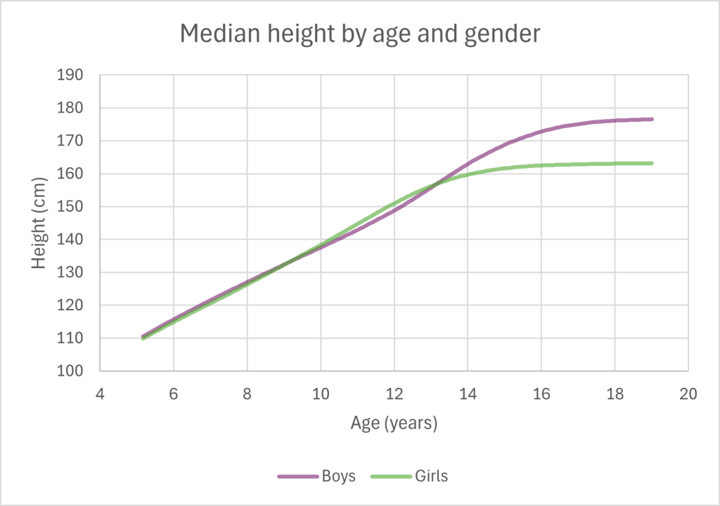
Alas, once the time series is extended, we see that the averages significantly diverge. Adding titles to the graph reveals why – it shows median height by gender from the ages 5 to 19:
Growth reference data from WHO; see percentiles for girls and boys xlsx files over here
Around age 9, the median girls’ height begins to exceed boys’, the difference peaking at about 12 years old. Then the difference in medians decreases until around 13 when boys’ median height begins to exceeds girls’.
Clearly, if we wanted to evaluate, e.g., an intervention to boost children’s height, we wouldn’t compare the mean height of one gender with another as control. The biological processes underpinning gender differences in pubertal growth spurt are well-known. However, diff-in-diffs is often applied in situations where much less is known about how changes occur over time.
As this example illustrates, the more we know about the topic under investigation and the more covariates we have at our disposal for choosing comparison units, the better our causal estimates using diff-in-diffs are likely to be. Diff-in-diffs can also be combined with matching or weighting on covariates to help construct a comparison group such that parallel trends is more likely to hold; see, e.g., Huntington-Klein (2022, Section 18.3.2).
Thanks very much to Thomas Aston (2024) for critical engagement in the Evaluation journal:
“… there were somewhat more thoughtful debates on the integration of experiments with theory-based evaluation. Of course, this is not a new discussion, but it reemerged, as I discussed in Randomista mania (Aston, 2023c), during a Kantar Public (2023) (now Verian) webinar on ensuring rigor in theory-based evaluation. In the United Kingdom, the Magenta Book guidance from HM Treasury (2020) includes a decision tree which implies, to some readers, that experimental designs cannot be theory-based. During the event, Alex Hurrell pointed out that theory-based evaluation and experimental methods are not necessarily irreconcilable. To this end, Andi Fugard (2023) wrote a blog arguing that “counterfactual” is not synonymous with “control group” and later conducted a thoughtful webinar for the UK Evaluation Society (2023) on challenging the theory-based counterfactual binary. In my view, Fugard is right that there is not a strict binary which implies that counterfactual approaches should not be theory-based. They have been moving in that direction for years (White, 2009). But perhaps the decision tree is less about the benefits of integrating theory into counterfactual approaches and more about the epistemic, practical, and ethical limits of experimental impact evaluation approaches and the importance of exploring alternative options when they are neither possible nor appropriate.”
I wish I shared Thomas’s optimism that the theory-based/counterfactual binary is already blurring. My reading is, the original 1975 definition of theory-based evaluation was inclusive and still is for those in the theory-driven camp (e.g., Huey Chen‘s work). But in many UK evaluation contexts, theory-driven is synonymous with contribution analysis, qualitative comparative analysis, and process tracing, applied to qualitative data. RCTs and QEDs are not allowed. There are notable exceptions.
Randomised controlled trials (RCTs) are an instance of the counterfactual kind of impact evaluation and contribution analysis of the theory-based kind. For example, the UK’s Magenta Book recommends using theory-based evaluation if you can’t find a comparison group (HM Treasury, 2020, p. 47). The founding texts on contribution analysis present it as using a non-counterfactual approach to causation (e.g., Mayne, 2019, pp. 173–4). In December 2023, I gave a talk to the UK Evaluation Society (UKES) exploring what happens if we challenge this theory-based/counterfactual binary. This post summarises what I said.
Good experiments and quasi-experiments are theory-based
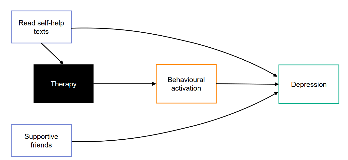
Theory is required to select the variables used in RCTs and quasi-experimental designs (QEDs); that is, to decide what data to gather and include in analyses. We need to peek inside the “black box” of a programme to work out what we are evaluating and how. These variables include outcomes, moderators, mediators, competing exposures, and, in QEDs, confounders.
This diagram denotes a causal directed acyclic graph (causal DAG). Therapy is conjectured to lead to behavioural activation, which alleviates depression. Supportive friends are a “competing exposure” that can alleviate depression. Reading self-help texts is a confounder as it predicts both whether someone seeks therapy and their outcomes, so this (made up) model is of a quasi-experimental evaluation.
In QEDs, many different model structures are compatible with the data. The slogan “correlation doesn’t imply causation” can be reformulated as A causes B and B causes A are Markov equivalent if all we know is that A and B are correlated. The number of models that are Markov equivalent rises exponentially as the number of variables and statistical associations increases. Theory is needed to select between the models: the data alone cannot tell us.
Although RCTs give us an unbiased estimate of an average treatment effect, that is, the average of each individual’s unmeasurable treatment effect (difference between measured actual outcome and counterfactual outcome), they cannot tell us what that difference represents. To do that, we need a theory of the ingredients and processes in the two programmes being compared; for example, what are the similarities and differences between CBT and humanistic counselling or whatever “treatment as usual” is in practice.
Counterfactual evaluations do not need a comparison group
There is a long history of research on counterfactual reasoning in the absence of a control group. How should we determine the truth of a counterfactual such as “If Oswald had not killed Kennedy, no one else would have” (e.g., Adams, 1970)? Clearly we ponder statements like these without running violent RCTs. Another strand of research investigates how children, adults, and animals perform counterfactual reasoning in practice (e.g., Rafetseder, et al., 2010). This research on non-experimental counterfactual reasoning includes literature in evaluation, for instance by White (2010) and more recently Reichardt (2022).
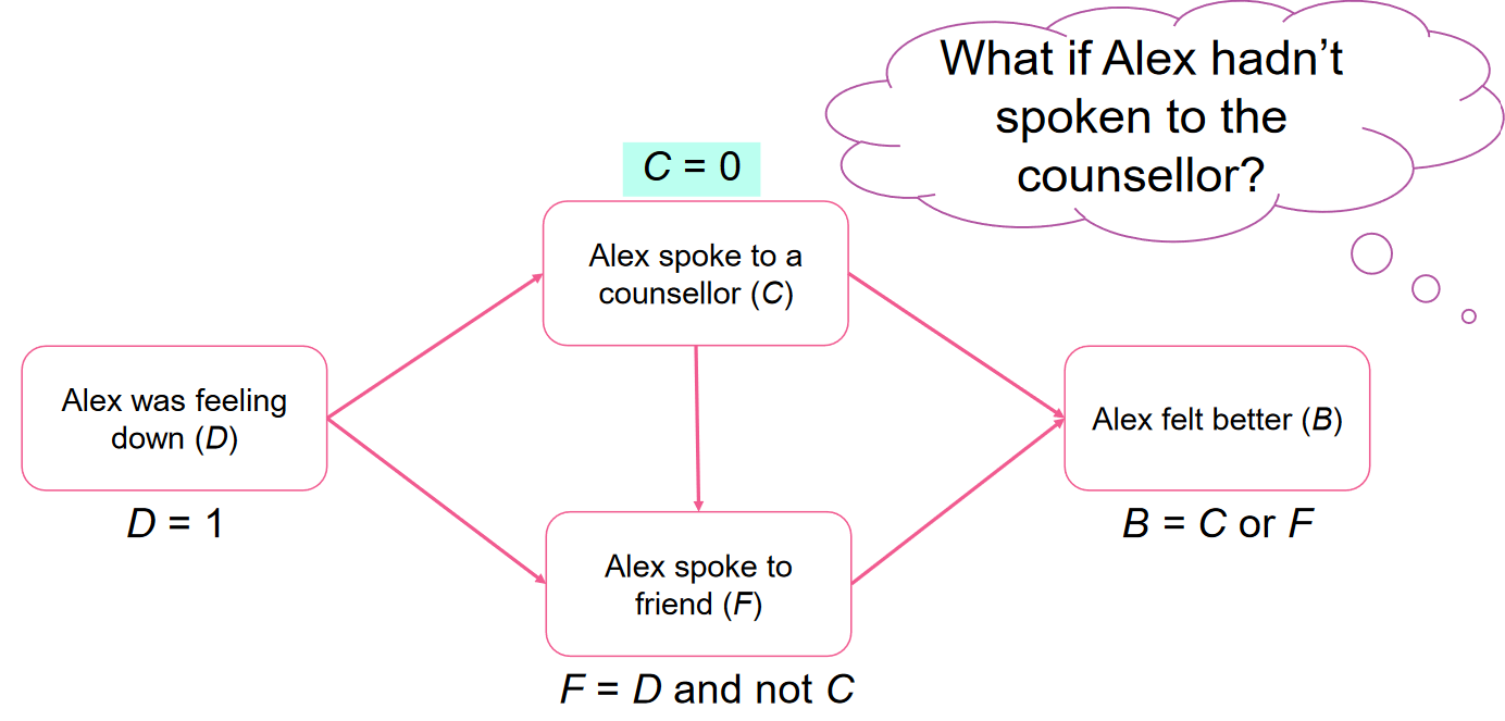
Halpern (2016) introduces a formal framework for defining causal relationships and estimating counterfactual outcomes, regardless of the sources of evidence. The diagram below illustrates the simplest version of the framework where causes and effects are binary. Equations, annotating each node, define the causal relationships and allow counterfactual outcomes to be inferred.
This is one of the models I used to illustrate counterfactual inference without a comparison group. In the factual situation, Alex was feeling down, spoke to their counsellor, and then felt better. In this counterfactual scenario, we are exploring what would have happened if Alex hadn’t spoken to their counsellor. In this case, they would have spoken to their friend instead and again felt better. Although there is no difference between the factual and counterfactual outcome, Halpern’s framework allows us to infer that Alex speaking to the counsellor was an actual cause of Alex feeling better.
This provides a concrete illustration of why RCTs and QEDs are unnecessary to reason counterfactually; however, the causal model obviously must be correct for the correct conclusions to be drawn, so one might reasonably ask what sorts of evidence we can use to build these models and persuade people they are true. There is also hearty debate in the literature concerning what constitutes an “actual cause” and algorithms for determining this are fiddly to apply, even if it is assumed we have a true model of the causal relationships. I explored Halpern’s approach in a previous blog post.
Summary
The original definition of theory-based evaluation by Fitz-Gibbon and Morris (1975) included the full range of approaches, qualitative and quantitative – including RCTs and QEDs. Many others follow in the tradition. For instance, Weiss (1997, p. 512) cites path analysis (a kind of structural equation model) as being “conceptually compatible with TBE [theory-based evaluation] and has been used by evaluators”. Chen and Rossi (1980) explain how theory-based (what they term theory-driven) RCTs that include well-chosen covariates (competing exposures) yield more precise estimates of effects (reducing the probability of Type II error), even though those covariates are not needed to control Type I error. Counterfactual queries do not need a comparison group. They do need a model of how facts came about that can be modified to predict the counterfactual outcome.
Challenging the theory-based/counterfactual binary does not mean that all evaluations are the same. There can still be variation in the strength of evidence used to develop and test theories and how well theories withstand those tests. However, taking a more nuanced view of the differences and similarities between approaches leads to better evaluations.
Fitz-Gibbon, C. T., & Morris, L. L. (1975). Theory-based evaluation. Evaluation Comment, 5(1), 1–4. Reprinted in Fitz-Gibbon, C. T., & Morris, L. L. (1996). Theory-based evaluation. Evaluation Practice, 17(2), 177–184.
Halpern, J. Y. (2016). Actual causality. The MIT press.
Excited to discover a triple of 2024 publications that use the broader conception of theory-based evaluation that includes trials and quasi-experiments, as the term was introduced by Fitz-Gibbon and Morris (1975) and used by, e.g., Chen and Rossi (1980), Coryn et al., (2011), Weiss (1997), Funnell and Rogers, P. J. (2011), Chen (2015), and many others.
I hope the next Magenta Book update has a more nuanced approach that includes RCTs and QEDs under theory-based, alongside, e.g., QCA and uses of Bayes’ rule to reason about qual evidence.
Chen, H.-T., & Rossi, P. H. (1980). The Multi-Goal, Theory-Driven Approach to Evaluation: A Model Linking Basic and Applied Social Science. Social Forces, 59, 106–122.
Chen, H.-T., & Rossi, P. H. (1983). Evaluating With Sense: The Theory-Driven Approach. Evaluation Review, 7(3), 283–302.
Chen, H. T. (2015). Practical program evaluation: Theory-driven evaluation and the integrated evaluation perspective (2nd edition). Sage Publications.
Coryn, C. L. S., Noakes, L. A., Westine, C. D., & Schröter, D. C. (2011). A systematic review of theory-driven evaluation practice from 1990 to 2009. American Journal of Evaluation, 32(2), 199–226.
Fitz-Gibbon, C. T., & Morris, L. L. (1975). Theory-based evaluation. Evaluation Comment, 5(1), 1–4. Reprinted in Fitz-Gibbon, C. T., & Morris, L. L. (1996). Theory-based evaluation. Evaluation Practice, 17(2), 177–184.
Funnell, S. C., Rogers, P. J. (2011). Purposeful Program Theory: Effective Use of Theories of Change and Logic Models. Jossey-Bass.
Weiss, C. H. (1997). How can theory-based evaluation make greater headway? Evaluation Review, 21(4), 501–524.
“The preceding paragraph illustrates a procedure that statisticians of all schools find important but elusive. It has been called the interocular traumatic test; you know what the data mean when the conclusion hits you between the eyes. The interocular traumatic test is simple, commands general agreement, and is often applicable; well-conducted experiments often come out that way. But the enthusiast’s interocular trauma may be the skeptic’s random error. A little arithmetic to verify the extent of the trauma can yield great peace of mind for little cost.” (Edwards, Lindman, & Savage, 1963, p.217, who attribute the “test” to J. Berkson, personal comm., 14 July 1958)
Edwards, W., Lindman, H., & Savage, L. J. (1963). Bayesian statistical inference for psychological research. Psychological Review, 70(3), 193.
‘In TBE [theory-based evaluation] practice […] theory as represented is not specific enough to support causal conclusions in inference […]. For example, in contribution analysis “causal assumptions” refer to a “causal package” consisting of the program intervention and a set of contextual conditions that together may explain an observed change in the outcome […]. In realist evaluation, the causal mechanisms that are triggered by the intervention are specified in “configuration” with their context and the outcome. Often, however, the causal structure of the configuration is not clear […]. Moreover, the main TBE approaches to inference do not have standard practices, conventions, for treating bias in evidence […].
‘TBE practitioners may borrow from other methods to test theoretical assumptions […]. Sometimes TBE employs regression analysis or quasi-experimental propensity score matching in inference (our running example in this article of an actual TBE program evaluation does so).’