M136279841

The largest known prime number was found on 12 Oct 2024 and is \(2^{136,279,841}−1\). It has the catchy name M136279841. You can download its digits in a zip file from a link in this press release.

I felt compelled to have a look at M136279841; however, it has 41,024,320 digits. So, I made do with looking at its first and last three digits (881, 551) and a plot of how frequent each digit is, using R. Code here.

There’s no evidence that any digit is more frequent than another, \(\chi^2(9) = 5.3\), \(p = .8\).

How p-values are distributed if the null hypothesis is true

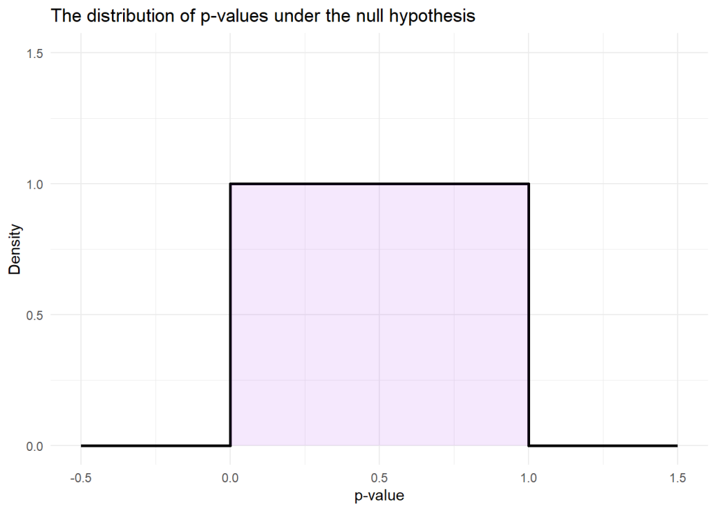
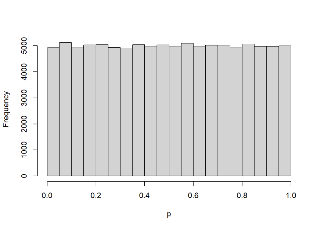
Here’s something random: how p-values are distributed if the null hypothesis is true. It’s the uniform distribution over the unit interval, [0, 1]. So every p-value between 0 and 1 is equally likely if the null hypothesis is true.

Here’s some R code to simulate:

null_distro <- function() {
x <- rnorm(100)
y <- rnorm(100)
t.test(x, y)$p.value
}
replicate(100000, null_distro()) |>
hist(main = "", xlab = "p")

Strings to vectors in R

Strings in R are difficult to use as the characters aren’t exposed, so you probably often write a function like this, to get a vector of characters:

\(x) strsplit(x, split = "")[[1]]

I’ve just discovered that this function is called chars in the newish {charcuterie} package. It also has its own class and a print method, so still prints like a string but works as a vector.

> "strawberry" |> charcuterie::chars() |> rev()
[1] "yrrebwarts"

Y in R

I’m delighted that R can implement the “paradoxical” Y combinator, so it’s possible to implement recursion using anonymous functions. Not sure why you’d want to, other than to reminisce about computation theory lectures, but onwards…

For instance, 5! is the one-liner:

(\(f) (\(x) f(x(x)))(\(x) f(x(x)))) (\(f) \(n) if (n == 0) 1 else n * f(n - 1)) (5)

Adding some names to that mess shows how absurd it is.

Here’s Y:

Y <- \(f) {
g <- \(x) f(x(x))
g(g)
}

Factorial, in a form to pass to Y:

fact <- \(f) \(n)
if (n == 0) 1 else n * f(n - 1)

Note how the f argument is used to recurse, rather than fact, as you’d usually do recursion.

Y(fact)(5) then gives 5! = 120.

Two or more arguments

This also works for functions with more than one argument. The trick is, don’t think, just write recursive functions as usual but with an extra argument at the front for recursing (here I’m using Schönfinkelisation/Currying).

This is multiplication on the naturals using recursive additions:

mult <- \(f) \(x) \(y)
if (x == 0) 0 else y + f(x - 1)(y)

Y(mult)(6)(7) gives 42.

The uncurried version:

mult <- \(f) \(x, y)
if (x == 0) 0 else y + f(x - 1, y)

Y(mult)(6, 7)

And the curried mult as a one-liner, for completeness:

(\(f) (\(x) f(x(x)))(\(x) f(x(x)))) (\(f) \(x) \(y) if (x == 0) 0 else y + f(x - 1)(y)) (6) (7)

Recall

If you just want to use recursion in an anonymous function or ensure that your recursive functions are robust to renaming, you can also use Recall (thanks @klmr@mastodon.social for pointing this out).

5! is:

(\(n) if (n == 0) 1 else n * Recall(n - 1)) (5)

Analysing individually randomized group treatment trials with complex clustering in nested and crossed designs

Interesting paper by Jonathan Moyer, Fan Li, and others on the best ways to analyse individually randomised trials in which (1) participants share professionals such as therapists and case workers, (2) participants may interact with multiple professionals over the course of the trial, and (3) the nesting structure may differ between experimental conditions.

Sampling without replacement with specified marginal sampling probabilities

The {sampling} library by Yves Tillé and Alina Matei implements Brewer’s (1975) method – discussed above – as UPbrewer. Tillé’s (2023) review looks interesting too, cataloguing a bunch of incorrect methods and what to use instead.

References

Brewer, K.E.W. (1975), A simple procedure for sampling πpswor. Australian Journal of Statistics, 17, 166-172.

Tillé, Y. (2023). Remarks on some misconceptions about unequal probability sampling without replacement. Computer Science Review, 47, 100533.

Comparing {eefAnalytics} and {lmeInfo}

In multilevel analyses, it is often necessary to estimate a standardised mean difference (SMD) where the numerator is a covariate-adjusted mean difference and the denominator is the SD from a model without covariate adjustment.

I’m aware of two (frequentist, non-bootstrap) packages calculating an SMD and confidence interval in R. Here’s a comparison of them for simulated data.

Work in progress – different ways to calculate Hedges’ g in cluster RCTs

The problem is, you want to estimate g with a covariate-adjusted treatment effect in the numerator but unadjusted SD in the denominator and an uncertainty interval of some description.

Work in progress R code here – scroll to the bottom for a table comparing results. Use at own risk.

Here is also a comparison of {eefAnalytics} and {lmeInfo}.

Impact of prior distributions in a single predictor Bayesian regression model

An example using brm in the {brms} package to explore the impact of different priors. (The right answer is 2.) The chosen priors are along the columns and samples sizes on the rows (15 and 1500). The N(mean = 0, SD = 0.1) prior really breaks it.

Here’s the posterior distro for n = 1,000,000 with the extreme prior N(0, 0.1) – it’s beginning to include the true value…